Vibration of Thin Plates

The present section is concerned with systems possessing two dimensions which are large compared with the third, e.g. plates whose lengths and widths are much greater than their thicknesses. There are numerous applications of vibrating plates in electroacoustical equipment such as loudspeakers, microphones, earphones, ultrasonic transducers, etc. In addition, plates can be found as constituting elements in several mechanical systems such as cars, trains, aircraft, and machinery. Plates, considered as plane systems, are a particular case of shells, whose surface may be of any shape. The general theory of vibrations of shells, which constitutes a large branch of mechanics, has been discussed by Leissa [14]. In 1828, Poisson and Cauchy established, for the first time, an approximate differential equation for flexural vibrations of a plate of infinite extent, and Poisson obtained an approximate solution for a particular case of the vibration of a circular plate. The development by Ritz in 1909 of the method for calculating the bending of plates on the basis of the energy balance was an important advance. This method made it possible to solve more complicated cases of the vibration of plates having different shapes [11]. Further advances were accomplished by the accurate calculation of the vibration distribution in rectangular plates with uniform and mixed boundary conditions [15].

a) Free Vibrations of a Rectangular Plate

For the requirements of acoustical engineering, it is sufficient to consider the flexural vibrations of thin plates (λ>>h, where h is the thickness of the plate) to which we can apply an approximate method analogous to that employed for bar [11].

The assumptions are:

1. The transverse cross‐sections of the plate still remain plane in the presence of strains, and
2. Neither longitudinal nor transverse strains occur on the middle (neutral) plane.

These conditions are satisfied approximately when the flexural wavelength is at least equal to a six times the thickness h of the plate. Under this assumption, the wave equation for transverse vibration of the plate is [14]

(2.65)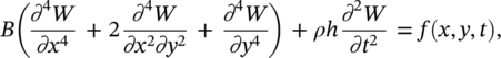

where W(x,y,t) is the instantaneous transverse displacement, ρ is the density of the plate, B = Eh³/12(1 − ν²) is the stiffness of the plate for bending, ν is the Poisson’s ratio, E is the modulus of elasticity (Young’s modulus) and f(x,y,t) are the external forces referring to unit surface area of the plate. The sum of the first three terms of Eq. (2.65) is a double Laplacian of W, ∇⁴ W, expressed in rectangular coordinates. It is useful to define the solution for steady‐state conditions as

(2.66)

where W₀(x,y) is the amplitude of the transverse displacement.

A vibrating structure, such as a plate, at any instant contains some kinetic energy and some strain (or potential) energy. The kinetic energy is associated with the mass and the strain energy is associated with the stiffness. In addition, any structure also dissipates some energy as it deforms. This conversion of ordered mechanical energy into thermal energy is called damping. A simple way to describe the energy loss is given by the analysis of the one‐dimensional system of Eq. (2.17). Thus, for sinusoidal vibration, use of a spring with an appropriately defined stiffness is completely equivalent to the use of an elastic spring and a dashpot. The internal losses in a plate arise not because of the motion of the plate as a whole body, but depend on the mutual displacements of the neighboring elements of the plate, and these are proportional to the changes in time of ∇⁴ W. Therefore, in order to account for energy dissipation in a plate, one may simply introduce a complex modulus of elasticity

(2.67)

where η is the internal loss factor of the plate. As an example, Figure 2.17 shows the computation of the velocity level response in decibels of the first resonance in a clamped‐clamped rectangular panel and the effect of varying its internal loss factor η.

The free vibration of plates has two important characteristics:

1. The velocity of propagation of flexural waves in the plate depends on frequency, and
2. The second component of the deflection, arising as a result of the stiffness of the plate, brings about additional changes, compared to a beam, in the distribution of the vibration.

As in the case of beams, plates can be fixed at their edges in various manners. Solutions for vibrating plates subjected to different boundary conditions have been discussed in several books for the 27 possible combinations [14, 17]. In this section we will discuss a uniform simply supported plate of length a and width b, mainly because this problem is illustrative and it has a closed‐form solution. In this case, the plate at its supports cannot perform motion perpendicular to its surface, but can rotate around the edge, and hence the displacement and bending moment are zero at the corresponding boundaries (see Eq. (2.55) for a beam)

(2.68)

The solution for the amplitude of flexural vibrations of a simply‐supported plate vibrating in mode (m,n), where m−1 and n−1 are the number of nodal lines in the x and y directions, respectively, can be obtained by separation of variables and is given by [14]

(2.69)

where A_mn is the modal amplitude, k_m = mπ/a, k_n = nπ/b and m and n are integers. Equation (2.69) gives the mode shapes of the simply‐supported plate. Figure 2.18 shows the first six mode shapes of a rectangular plate. Natural frequencies of each plate’s mode (m,n) are given by

(2.70a)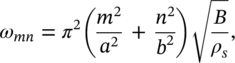

where ρ_s is the mass of the plate per unit surface area. Note that Eq. (2.70a) can be approximated by

(2.70b)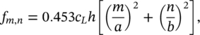

where f_m,n is the characteristic modal frequency (Hz) and c_L is the longitudinal wave speed in the plate material (m/s).

Thus, the total solution for the free vibration of a simply‐supported plate is

(2.71)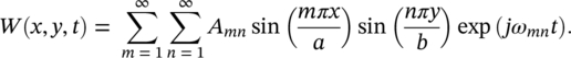

Note that for a square plate (a = b) ω_mn = ω_nm. Therefore modes (m,n) and (n,m) have the same frequency and they are called degenerate. This fact also happens when the length or width are integer multiple of each other.

EXAMPLE 2.12

Determine the natural frequency of the fundamental mode of a plywood board of thickness 8 mm, mass density 812.5 kg/m³, and dimensions a × b = 0.7 × 0.6 m².

SOLUTION

The plywood board has properties E = 6 × 10⁹ N/m², S = a × b = 0.7 × 0.6 m², and ν = 0.3. The mass of the plate per unit surface area ρ_s = ρ × h = 812.5 × 0.008 = 6.5 kg/m². and the bending stiffness B = Eh³/12(1 − ν²) = 6 × 10⁹(0.008)³/12 (1 − [0.3]²) = 281.3 N/m. Then, the fundamental mode (the lowest natural frequency) is given for m = n = 1. Replacing the values in Eq. (2.70a) yields

b) Forced Vibration of a Rectangular Plate

Let us assume that a distributed harmonic force acts on a rectangular plate (referred to unit plate area)

(2.72)

Under the influence of this force, a plate deflection W is produced with the distribution

(2.73)

The distribution of the deflection amplitude W₀ can be represented by the resultant of a series of sinusoidal vibrations. The frequency is equal to the frequency of free vibration of the plate, that is to say, the following equation must be satisfied [18]

(2.74)

where k_mn = ω_mn/c_b is the wavenumber of the (m,n) mode of free vibration, c_b is the velocity of bending waves in the plate and Ψ_mn are the dimensionless coefficients which determine the relative distribution in relation to the maximum amplitude of deflection.

Using the orthogonality of the function Ψ_mn and Fourier series, the resultant distribution of vibration on the rectangular plate is given by [16]

(2.75)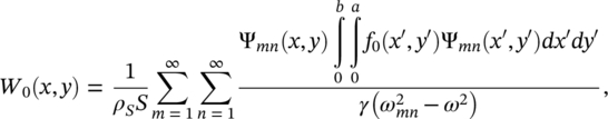

where (x′, y′) denotes the coordinates of the position of the force f (referred to unit plate area), with respect to which the integration is carried out over the surface area of the plate. The ω_mn are real numbers for a plate without losses. For the frequency of forced vibration ω = ω_mn, the amplitude of the deflection grows theoretically to infinity. In a plate with losses, ω_mn are complex numbers, as discussed in Section 2.4.3.

For example, for a simply‐supported rectangular plate, the distribution Ψ_mn (see Eq. (2.69)) is

(2.76)

and γ = 1/4. Then, we can obtain that for a point force F concentrated at the point (x₀, y₀)

(2.76)

The vibration velocity distribution on the rectangular plate can be obtained as

(2.77)

In practice, to calculate the plate response to a concentrated force, it is necessary to truncate the infinite summation. More complicated cases of boundary conditions have been studied in the literature [19].

All the theory presented above and the subsequent applications have been developed assuming light fluid loading, so that the plate response is not affected by the surrounding environment, which acts as added mass and radiation damping [20]. This criterion is not valid for submerged structures.

EXAMPLE 2.13

The numerical results for the velocity level at the coordinate point (x,y) = (0.04, 0.03) for a plywood board with properties E = 6 × 10⁹ N/m², ρ_S = 6.5 kg/m², a × b = 0.7 × 0.6 m², ν = 0.293 and η = 0.01 are presented in Figure 2.19. The reference velocity is 10⁻¹⁸ (m/s)². It is observed that excitation close to a corner excites more modes in the plate. Excitation at the middle point of the plate excites mostly the modes (m,n) where m and n are both even, while no contribution to the velocity level is included from modes having nodal lines passing through the center of the plate.