Tail Pipe Radiation Impedance, Source Impedance and Source Strength

10.8.1 Tail Pipe Radiation

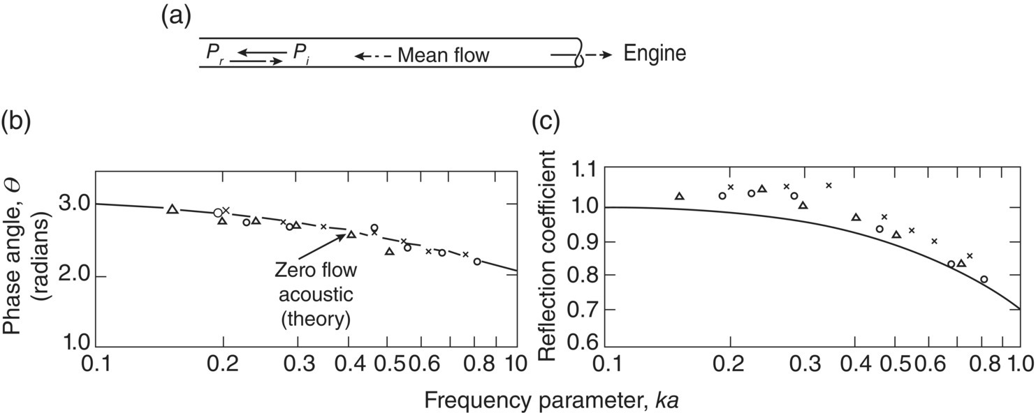
Early work on engine exhaust mufflers was hampered by a lack of knowledge of the reflection of waves at the end of the tail pipe. As Alfredson and Davies discuss [39], various assumptions have been made in the past about the magnitude and phase of the reflection (some researchers assumed the reflection coefficient R was zero and some, one). In 1948, Levine and Schwinger [67] published a rigorous, lengthy theoretical derivation of the reflected wave from an unflanged circular pipe. The solution assumes plane wave propagation in the pipe and no mean flow. In 1970, Alfredson measured the reflection coefficient R and phase angle θ of waves in an engine tail pipe using the engine exhaust as the source signal. The motivation was to determine if a mean flow and an elevated temperature had a significant effect on the zero flow reflection coefficient and phase calculated by Levine and Schwinger. Both the theoretical results of Levine and Schwinger and Alfredson’s experimental results are given in Figure 10.27. Alfredson’s experimental results show only a 3–5% increase in the reflection coefficient and virtually no change in the phase angle, as the flow and temperature increase to those conditions found in a typical engine tail pipe. Either Alfredson’s or Levine and Schwinger’s results for R and θ can be used to determine the tail pipe radiation impedance Z_r used in IL or sound pressure predictions (Eqs. (10.60) and (10.68)).

The sound pressure and volume velocity can be written as follows:

(10.69)

and

(10.70)

Then the ratio of the pressure and volume velocity at the tail pipe exit is given by dividing Eqs. (10.69) by (10.70). The radiation impedance Z_r is calculated from Eq. (10.71).

(10.71)

10.8.2 Internal Combustion Engine Impedance and Source Strength

Until the late 1970s, values of engine impedance used in predictions had been completely speculative. Values of Z_e, of ∞, ρc/S, and 0 were assumed by various workers in making IL calculations. Other experimenters tried to simulate these different values in their idealized experimental arrangements. Values of Z_e = ∞, and 0, correspond to constant‐volume velocity (current) and constant pressure (voltage) sources, respectively. Suppose the muffler and termination impedances shown in Figure 10.26 are lumped together as a load impedance, then Figure 10.26b and 10.26c reduce to Figure 10.28a and 10.28b, respectively.

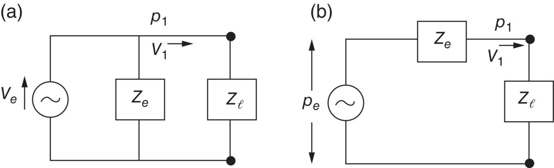
In the case of a volume velocity source, V₁ = V_e Z_e/(Z_e + Z_l) and if the internal impedance Z_e → ∞, V₁ → V_e. Thus, a constant‐volume velocity is supplied to the load, independent of its value (provided it remains finite). When Z_e → ∞, this source is known as a constant‐volume velocity source.

In the case of a pressure source, p₁ = p_e Z_l/(Z_e + Z_l) and if the internal impedance Z_e → 0, p₁ → p_e. Thus, a constant sound pressure is supplied to the load terminals, independent of the load impedance value (provided it remains finite also). When Z_e → 0, this source is known as a constant pressure source. Note that if Z_e = ρc/S in either model, that constant sources are not obtained in either model. These constant‐volume velocity and constant pressure sources are equivalent to constant current and constant voltage sources which are well known in electrical circuits (see, e.g. Reference [68]).

In the case of automobile engines, it is of course unlikely, in practice, that the engine impedance is approximately 0, ρc/S, or ∞. However, it could approach one of these values in certain frequency ranges. Some have even questioned the meaning of engine impedance since it must vary with time as exhaust ports open and close. There are at least three approaches to model the automobile engine source characteristics. Without directly using the concept of engine impedance as such, Mutyala and Soedel [69, 70], have used a mathematical model of a single‐cylinder two‐stroke engine connected to a simple expansion chamber muffler. The passages and volumes are treated as lumped parameters and kinematic, thermodynamic and mass balance equations are used. Good agreement between theory and experiment was obtained for the radiated exhaust noise.

Galaitsis and Bender [71] used an empirical approach to measure engine impedance directly. Using an electromagnetic pure tone source and by measuring standing waves in an impedance tube connected to a running engine they were able to determine the engine internal impedance. At low rpm the impedance fluctuated with frequency. However, at high rpm the impedance approached ρc/S at high frequency. Ross [72] has also used a similar technique.

A third approach to the determination of engine impedance (and source strength) is the two‐load method. This method is well known in electrical circuit theory.

Using the pressure source representation (see Figure 10.28b) and two different known loads Z_l and , two simultaneous equations are obtained:

(10.72)

(10.73)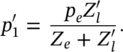

Eliminating p_e in Eqs. (10.72) and (10.73) gives:

(10.74)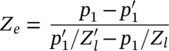

Substitution of Z_e in Eqs. (10.72) or (10.73) now gives the source strength p_e. Kathuriya and Munjal suggest using two different length pipes so that there is little change in back pressure and so that (presumably) the load impedances, and Z_l (comprised of straight pipe and radiation impedance) are well known [65]. In order to remove the necessity to measure p_l inside the tail pipe (where the exhaust gas is hot) it should be possible to measure the sound pressure radiated from the tail pipe p_r since this can be related to the pressure p_l in the straight pipe by equations, such as (10.64) and (10.67). Egolf [73] has used this two‐load method in the design of a hearing aid. Sullivan [30] has discussed the limitations of the method. Methods of measuring the internal impedance of sources are discussed further in Section 10.11.