Random Noise

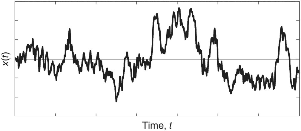
So far we have discussed periodic and nonperiodic signals. In many practical cases the sound or vibration signal is not deterministic (i.e. it cannot be predicted) and it is random in time (see Figure 1.5). For a random signal, x(t), mathematical descriptions become difficult since we have to use statistical theory [1, 7, 9]. Theoretically, for random signals the Fourier transform X(ω) does not exist unless we consider only a finite sample length of the random signal, for example, of duration τ in the range 0 < t < τ. Then the Fourier transform is

(1.6)

where X(ω,τ) is the finite Fourier transform of x(t). Note that X(ω) is defined for both positive and negative frequencies. In the real world x(t) must be a real function, which implies that the complex conjugate of X must satisfy X(−ω) = X^*(ω); i.e. X(ω) exhibits conjugate symmetry. Finite Fourier transforms can easily be calculated with special analog‐to‐digital computers (see Section 1.5).

EXAMPLE 1.2

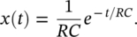
An R–C (resistance–capacitance) series circuit is a classic first‐order low‐pass filter (see Section 1.4). Transient response describes how energy that is contained in a circuit will become dissipated when no input signal is applied. The transient response of an R–C series circuit (for t > 0) is given by

Find the Fourier spectrum representation of this transient response.

SOLUTION

Substituting x(t) into Eq. (1.6) we obtain

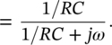
Therefore,

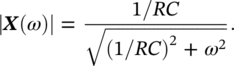
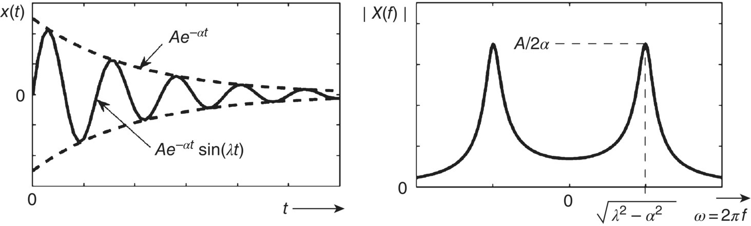
The transient response and its Fourier spectrum are shown in Figure 1.6.

EXAMPLE 1.3

The impulse response of a dynamic system is its output in response to a brief input pulse signal, called an impulse. The impulse response of the damped vibration of a one‐degree‐of‐freedom mass‐spring system of mass M, stiffness K, and coefficient of damping R (see Chapter 2 of this book) is given by

where A = (Mω_d)⁻¹, α = R/2 M and λ = ω_d is known as the damped “natural” angular frequency. Find the Fourier spectrum representation of this impulse response.

SOLUTION

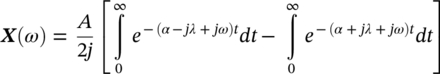
Using the mathematical property e^jθ = cos θ + j sin θ, we can write

. Then, Eq. (1.6) is

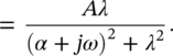
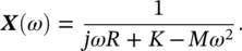
The impulse response and its Fourier spectrum are shown in Figure 1.7. We notice that replacing α and λ by the corresponding values in terms of the stiffness K, mass M, and damping constant R, of the damped mass‐spring system, the Fourier spectrum becomes (compare with Eq. (2.18))