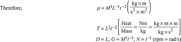
Let us consider the following variables for the performance of the compressor.
p3 = pressure at the outlet of diffuser
p1 = inlet pressure
T1 = inlet temperature
D = diameter
G = mass rate of flow
N = r.p.m of rotor
Then, p3 = f (p1, T1, D, G, N)
The following dimensions are chosen:
M = mass (kg), L = length (m), t = time (s)
Number of variables, n = 6
Basic dimensions, m = 3
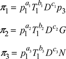
According to Buckingham’s Pi theorem, the number of dimensionless groupsm = n − m = 6 − 3 = 3
The three dimensionless groups are formed by combining p1, T1, and D with each of the remaining variables, so that
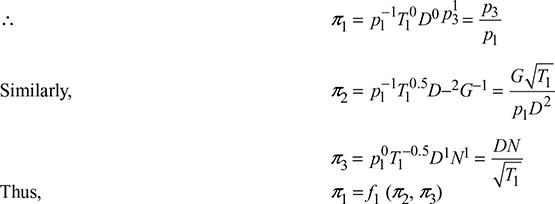
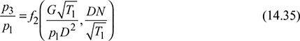
Substituting the basic dimensions for the variables in π1, we have
π1 = (M1L−1t−2)a1 (L2t−2)b1 Lc1(M2L−1t−2)1
For M, 0 = a1 + 1
For L, 0 = − a1 + 2b1 + c1 −1
For t, 0 = − a1 − 2b1 −2
From which, a1 = −1, b1 = 0, c1 = 0
For a given compressor under consideration, D = const.
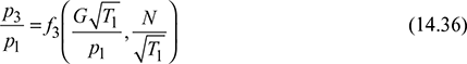

Similarly, the ratio ![]() can be formed to be function of the dimensionless groups of Eqs. (14.35) and (14.36). Similarly, if stagnation temperature and pressure are considered, the result will again be the same except that stagnation temperatures and pressures are substituted in place of static pressures and temperatures.
can be formed to be function of the dimensionless groups of Eqs. (14.35) and (14.36). Similarly, if stagnation temperature and pressure are considered, the result will again be the same except that stagnation temperatures and pressures are substituted in place of static pressures and temperatures.
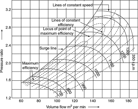
Figure 14.12 Pressure ratio v’s Volume flow rate
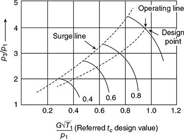
The performance of a given compressor or geometrically similar compressor can be plotted in terms of three dimensionless parameters provided dynamic similarity is maintained. Fig. 14.11 shows a plot of ![]() against
against ![]() and
and ![]() . The operating line is the locus of the points of maximum efficiency at various values of
. The operating line is the locus of the points of maximum efficiency at various values of ![]() . The surge line represents the stable operation, the region to the right of the surge line being for stable conditions.
. The surge line represents the stable operation, the region to the right of the surge line being for stable conditions.
The performance of the compressor has been plotted in terms of volume flow rate and pressure ratio in Fig. 14.12.
Leave a Reply