Power generation plants around the world often employ gas turbines and other industrial equipment, which need to be muffled. The inlets and exhausts of large fans and blowers in buildings must also be muffled. Very often large industrial mufflers have to be designed individually for specific applications to achieve optimum performance and acceptable physical size. Normally high sound attenuation over a wide frequency band is required. In addition, the pressure drop in the flow along the muffler should be small and the muffler’s physical dimensions made as small as possible. To meet each of these technical requirements individually is not technically difficult, but to meet all three requirements at once is very difficult. For example, a small muffler designed to have a large attenuation will result in one with a large pressure drop, or one with attenuation in only a narrow frequency band. The amount of attenuation required depends not only on the size and type of the industrial equipment to be muffled, but on the proximity of fans and blowers to occupants of buildings or those living in residential communities nearby. Thus, it is important that the properties and size of such mufflers be determined properly in the design stage. As discussed by Vanderburgh [141], designs must be concerned with the increased diversity of equipment and air‐conditioning systems to be muffled. There is now more awareness of the problems of low‐frequency noise and sound spectrum imbalance in buildings.
Figure 10.74a gives a sketch of a duct lined on two sides along with the symbols and terminology normally used. Parallel‐baffle mufflers consist of multiple side‐by‐side arrangements of ducts lined on two sides. See Figure 10.74b. Figure 10.74c shows a circular muffler. There is not one universally‐accepted method to predict the attenuation of parallel‐baffle and circular‐section mufflers. If a duct is lined on all four sides, the total attenuation may be assumed to be the sum of the attenuation of each pair of sides evaluated independently [14, 15]. The attenuation of a circular duct can be assumed to be equal to a square duct lined on all four sides and having a cross‐sectional area equal to that of the circular duct. There are several empirical schemes with associated charts and theoretical studies, which can be used to determine the attenuation of parallel‐baffle mufflers.
The studies assume that the attenuation in a duct can be related to the percentage of open area, (% open area/duct cross‐sectional area). The early study of Sabine [128] found that the attenuation could be related to the Sabine absorption coefficient αsab (raised to the power 1.4) and the ratio of the perimeter P of the duct cross‐section to the open area A. This empirical result may be explained by assuming the acoustic energy in the duct length l is exposed to the surface area Al of the absorbing material which has an absorption coefficient αsab. Although this result becomes increasingly inaccurate at the frequency increases, it is still useful at very low frequency (e.g. less than 200 Hz.)
Embleton was one of the first to publish a chart in 1971 to predict the attenuation of parallel‐baffle mufflers [8]. Embleton’s chart was based on the then unavailable results of Ingard and his unpublished computer program, which remained unpublished until 1994 [149]. Ver also produced design charts in 1982 for the attenuation of parallel‐baffle mufflers [136]. His results were republished in the book edited by Beranek and Ver in 1992 and also in the later version of this book edited by Ver and Beranek in 2006. Bies, Hansen, and Bridges also produced a family of parallel‐baffle attenuation prediction charts, which were also republished in the Bies and Hansen book [14, 150]. Bogdanovic [145] has written a useful review of all of these parallel‐baffle muffler attenuation prediction methods with the exception of the ones by Bies and Hansen [14] and Ramakrishnan and Watson [151].
Various authors have used different symbols for flow resistance, baffle thickness, baffle spacing, etc. The symbols used are summarized in Table 10.3. In Sections 10.14.1–10.14.7 the original symbols used by these authors in the figures and text in this chapter have not been altered. To avoid any confusion, the reader should consult Table 10.3 and/or the original references.
Table 10.3 Symbols used by various authors in parallel‐baffle mufflers.
| Symbol | Flow Resistance | Flow Resistivity | Normalized Flow Resistance | Liner Thickness, m | Gap Between Liners, m | Frequency Parameter |
|---|---|---|---|---|---|---|
| Author | ||||||
| Embleton | Rl | R | Rt/ρc | t | ly | ly/λ |
| Ver | R | R1 | R1 d/ρc | d | 2h | 2hf/c |
| Ingard | — | — | R | d | D | D/λ |
| Bies and Hansen | R | R1 | R1 d/ρc | t | 2h | 2h/λ |
| Mechel | r0 d | r0 | r0 d/Z0 | 2d | 2h | fh |
| Ramakrishnan and Watson | rc d | r0 | r0 d/ρc | d | h | μ = 2hf/c |
10.14.1 Embleton’s Method
Embleton’s chart is given in Figure 10.75. The parameters required to use the chart are the % open area, the spacing between the baffles ly and the wavelength of sound λ. The airflow temperature is assumed to be 25 °C. The curves give values of the normalized flow resistance parameter Rt/ρc, where R is the flow resistance per unit thickness, t is the material thickness and ρc the air characteristic impedance. However, Embleton states that the open area has the dominant effect and that the curves are not very sensitive to changes in the flow resistance per unit thickness, R. Thus, Embleton suggests that the curves in Figure 10.75 may be used over an appreciable range of values of R (from one half to twice the nominal values of Rt/ρc given in Figure 10.75) [8]. The attenuation parameter Aly given in Figure 10.75 is the attenuation per length of duct equal to the duct width ly. Thus, the attenuation of a duct of length le is Aly (le/ly) dB.
Embleton’s chart remains useful because of its simplicity. However, several other authors have now produced attenuation versus frequency prediction curves for parallel‐baffle mufflers [136] in which baffle thickness and spacing, mean flow and material resistivity are considered separately. The prediction schemes normally present results for the attenuation for a muffler having a length equal to the spacing between baffles (termed duct “width” or “height”) as ordinate. The abscissa is usually the non‐dimensionalized frequency, (half duct width h divided by wavelength λ). The authors’ own symbols and terminology are used in the following sections of this review.
10.14.2 Ver’s Method
In 1982, Ver published a series of five charts for open areas ranging from 16.6 to 83% to predict the attenuation of parallel‐baffle mufflers [136]. Three of these curves with % open areas ranging from 33 to 66% were subsequently republished in two books [11, 12]. See Figure 10.76. Figure 10.76 shows that the attenuation does not depend strongly on the normalized flow resistance R = R1 d/ρc in the range from R = 1 to 5. Although designers may be tempted to reduce the % open area to broaden the high attenuation region, this can cause problems. When the % open area is reduced, the mean flow velocity will need to increase correspondingly unless the total muffler size is increased. Higher mean flow velocity causes increased flow noise and greater pressure drop with an increased loss in system efficiency.
Ver [11, 12, 136] also published a chart showing the attenuation TLh (equivalent to the Aly of Embleton) against the frequency parameter 2 hf/c (equivalent to 2 h/λ) illustrating the effect of variations in the % open area. Figure 10.77 shows the very strong dependence of the normalized attenuation on the % open area for a value of the normalized flow resistance parameter R = 5. As the value of the % open area is reduced from 83% to 16.6% the region of high attenuation is broadened substantially.
10.14.3 Ingard’s Method
As discussed before, Embleton states that his prediction scheme for parallel‐baffle mufflers is based on unpublished results of Ingard. Ingard later published his results for such mufflers in 1994 and it is of interest to compare them with Figure 10.75 published by Embleton. Ingard’s results given here are for a rectangular duct with a non‐locally reacting porous layer on one side only [149]. See Figures 10.78 and 10.79. They are with the percentage open area varying from 20 to 70%. Ingard has also similar results for locally reacting ducts lined on one side only but with the open area varying only from 20 to 40%. The theoretical model for the non‐locally reacting duct is more complicated than for a locally reacting duct. Ingard provides a computer program along with his book, but unfortunately the programs are designed to run using the DOS language and are difficult to implement with modern computers. Although Ingard’s results are for ducts lined on one side only, those for parallel‐baffle mufflers may be inferred by assuming his result applies to a duct lined on both sides of double the width (i.e. 2D.) Locally reacting linings are difficult to implement in practice since multiple partitions need to be embedded in the absorbing layer periodically. However, Ingard’s results for non‐locally and locally reacting liners for the same % open area and normalized flow resistance differ from each other only marginally in most cases.
10.14.4 Bies and Hansen Method
Bies and Hansen give a series of curves for the attenuation rate of ducts lined on two sides. They assume two cases: (i) locally reacting absorbent liners, and (ii) non‐locally reacting liners (which they term bulk‐reacting.) They also give results for flow (M = 0.1) in the direction of sound propagation and flow in the opposite direction to the sound propagation (M = −0.1). Their results suggest that the assumption of locally reacting liners leads to a peak attenuation somewhat higher than for non‐locally (or bulk) liners. The positive or negative flow direction seems to affect the magnitude of the peak attenuation much more than shifting the frequency of the peak attenuation (See Figures 10.80 and 10.81.). One explanation is that when the flow is in the same direction as the sound propagation, the convection reduces the time the sound has to be absorbed and so the attenuation is also reduced accordingly. An alternative explanation preferred by Hansen is that due to friction along the duct walls, the speed of the flow is maximum in the duct center and reduces as the duct wall is approached. This results in sound rays being refracted away from the duct walls when sound is traveling in the same direction as the flow and refracted into the walls when sound is traveling in the opposite direction to the flow, resulting in more sound energy being absorbed.
 is the liner thickness, h is the half width of the airway, R1 is the liner flow resistivity. Locally reacting liner with no limp membrane covering (density ratio σ/ρh = 0). Zero mean flow (M = 0) (after Bies and Hansen) [14, 15].
10.14.5 Mechel’s Design Curves
Mechel has published a series of design curves for parallel‐baffle mufflers. See Figures 10.82 and 10.83. His predictions are assumed to be for locally reacting lining material since partitions are shown in the linings. Figure 10.82a shows the effect of varying the normalized flow resistance r0 d/Z0 while the open area ratio OA is held constant at 50% (d/h = 1). Here the characteristic impedance ρc is replaced with the symbol Z0. The first thickness resonance of the baffle is observed clearly for a small normalized flow resistance r0 d/Z0 = 1.5. It is smoothed out as the normalized resistance is increased to 3.0 and disappears entirely when the resistance is increased to 6.0. As the flow resistance increases, so does the attenuation increase at low frequency, which is important in real applications. Figure 10.82b shows the effect of varying the normalized flow resistance with the open area ratio OA kept at 33% (d/h = 2). The first thickness resonance is moved to a lower frequency and the low frequency attenuation is increased compared with the d/h = 1 case. Figure 10.82c shows the effect of keeping the normalized flow resistance constant r0 d/Z0 = 2 while the open area ratio is varied from OA = 66 to 25%. As predicted by other researchers, the increase in open area tends to broaden the attenuation curve while causing only a small reduction in peak attenuation. Increasing the thickness ratio d/h is the most effective way of obtaining high values of attenuation at low frequency [152]. However, care must be taken, since increasing d/h will also lead to higher values of pressure drop or increase in muffler size. Figure 10.83 provides a very encouraging comparison between Mechel’s prediction and measurements. Unfortunately, the flow resistance is not given for this case.
10.14.6 Ramakrishnan and Watson Curves
Ramakrishnan and Watson present a series of curves for the attenuation rates for lined parallel‐baffle rectangular mufflers [151]. See Figures 10.84 and 10.85. The authors define the normalized frequency μ = 2fh/c and normalized flow resistance R = r0 d/ρc. The finite element approach which they use also considers multimodal acoustic propagation. The sound‐absorbing liners are assumed to be bulk‐reacting (non‐locally reacting) and thus the model allows for sound propagation in the lining material itself. The authors also compare their predictions with experiment and obtain good agreement except in some cases where N1 = d/h is small. (See their published tabulated results.)
In the example following, the attenuations predicted by the different design curves in Sections 10.14.1–10.14.6 are compared. Some of the design methods can include the effect of temperature and mean flow (usually in terms of Mach number M). Since other methods do not make allowance for mean flow, it will be assumed to be zero in this example. The main effect of the temperature of the mean flow is to change the speed of sound c and thus the wavelength λ = c/f used in the non‐dimensional frequency calculation.
The number of baffles and parallel duct sections needed depends on providing sufficient ducting to accommodate the volume flow rates of the fans, blowers, turbines etc. The number of parameters required includes the mean flow resistance of the absorbing material, the thickness of the baffles, d, and the spacing between them, 2 h.
EXAMPLE 10.7
A parallel‐baffle muffler consists of baffles each 0.1 m thick with a spacing of 0.1 m between each set of baffles. Calculate the attenuation of a muffler of length 1 m. Assume the normalized flow resistance of the absorbing material is 5.0.
SOLUTION
The results are shown in Table 10.4.
The results of the worked Example 10.7 show that the six different methods illustrated in Table 10.4 produce similar results with the greatest predicted attenuations in the 1000–4000 Hz range. Choosing accurate values from the curves for attenuation at low frequencies in the range 125–250 Hz and at high frequencies in the range 4000–8000 Hz is difficult because the curves are steeply sloping and interpolation must be used with the non‐dimensional frequency scale. Mechel’s curves [152] can be used with some confidence since they have experimental confirmation with measurements made in a very high‐quality facility in Stuttgart, Germany. The Ramakrishnan/Watson curves agree very closely with Mechel’s curves except for the peak values at 2000 Hz. Although Bogdanovic presents one experimental result [145], which was in good agreement with Embleton’s curves, Embleton’s method seems to overpredict the attenuation compared with the five other methods. Ingard’s curves are very steeply sloping at high frequency, leading to the prediction of very small attenuation values for 4000 and 8000 Hz.
Table 10.4 Calculated values of muffler attenuation from methods given in Sections 10.14.1–10.14.6.
| Method | Frequency, Hz | 125 | 250 | 500 | 1000 | 2000 | 4000 | 8000 |
|---|---|---|---|---|---|---|---|---|
| 2 h/λ | 0.036 | 0.073 | 0.146 | 0.292 | 0.584 | 1.167 | 2.334 | |
| Embleton | Attenuation, dB | 2 | 9 | 19 | 27 | 32 | 29 | 13 |
| Ver | Attenuation, dB | 1 | 3 | 8 | 18 | 26 | 20 | 4 |
| Ingard | Attenuation, dB | 3 | 7 | 12 | 20 | 22 | 3 | 1 |
| Bies/Hansen | Attenuation, dB | 1 | 3 | 7 | 15 | 27 | 20 | 5 |
| Mechel | Attenuation, dB | 1 | 3 | 10 | 20 | 28 | 24 | 6 |
| Ramakrishnan/Watson | Attenuation, dB | 1 | 2 | 10 | 20 | 25 | 24 | 6 |
10.14.7 Finite Element Approach for Attenuation of Parallel‐Baffle Mufflers
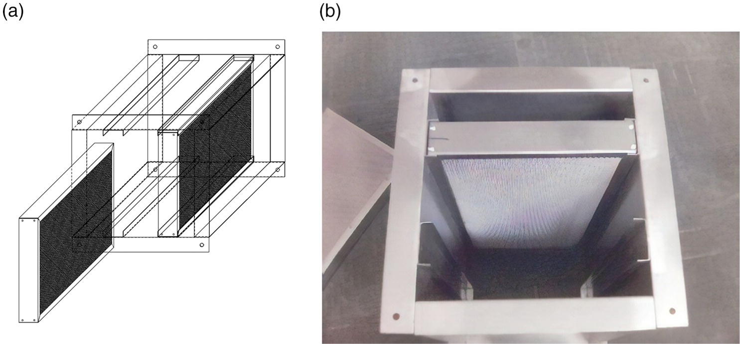
Astley and Cummings [140] presented a family of attenuation prediction curves for lined ducts and parallel‐baffle mufflers using finite elements in 1987. However, these curves are not particularly easy to use. More recently, in 2012, Borelli and Schenone [143] also used FEM to predict the attenuation of parallel‐baffle mufflers. They used a commercial software for the FEM using a brick mesh and the PARDISO solver which allowed analysis up to 8000 Hz much faster than with the use of traditional solvers. They claim very good agreement between company catalog attenuations given for commercial mufflers and their predictions. Figure 10.86 shows one comparison between their predictions and their own measurements. The muffler that they tested using EN ISO 11691 and EN ISO 7235 standards is given in Figure 10.87. However, another muffler model FCR SQ‐A‐110‐600 they tested produced somewhat less satisfactory prediction results with an error in their predictions of the order of about 3 dB at 2000 Hz.
Three additional effects should be accounted for:
- Discontinuities at the beginning and end of the lined duct section of the muffler. Although normally the muffler entrance and exit is made continuous with the main ductwork, the soft lining presents a sudden expansion in cross‐section, a similar effect happens at the exit, where the sound field experiences a sudden contraction. These effects can be accounted for by considering the muffler as a lined expansion chamber. A correction for parallel‐baffle muffler attenuation can be made using the curves given by Embleton [8]. Embleton’s correction curves are repeated in the books by Bies and Hansen [14] and Munjal [15].
- Pressure drop. Embleton, Bies and Hansen, and Mechel discuss the problems of pressure drop (sometimes called back pressure) in muffler designs [8, 14, 15]. Embleton describes three main sources, including the inlet and exhaust junction reflections, turbulent‐flow creation, and additional end expansion effects [8]. Mechel describes the same three sources of pressure drop and characterizes them in terms of drag coefficients relative to the pressure. Mechel also stresses that it is important to streamline the leading edges of the baffles [152]. Ver and Beranek discuss how the pressure drop can be estimated [15].
- Flow effects including flow temperature. As already discussed, flow effects the effective sound wavelength in the muffler like a Doppler shift affecting the absorption of the sound [8, 12, 15, 152]. The temperature of the mean flow effects the speed of sound and thus also the effective frequency. The reader is directed to other references for more detailed discussions of these effects [8, 12, 15, 152].
Leave a Reply