Measurement of Sound Intensity

The measurement of sound intensity is much more complicated than the measurement of sound pressure. In general, it requires the simultaneous measurement of sound pressure and particle velocity. This needs the use of at least two transducers. There are currently three main methods in use:

1. The so‐called p–p method, in which the particle velocity is determined from the sound pressure difference between two closely‐spaced microphones and the sound pressure is taken to be the average of the two microphones signals.
2. The p–u method, in which the particle velocity is determined by a particle velocity transducer and the sound pressure is obtained with a pressure microphone.
3. The p–a method, in which the surface velocity of a vibrating surface is obtained by integrating the signal from a surface‐mounted accelerometer and the sound pressure is measured with a pressure microphone located close to the accelerometer.

The first p–p method is well established and has been in use now for almost 40 years and will be discussed in detail first. It is currently the dominant way of measuring sound intensity.

8.6.1 The p–p Method

The most successful measurement principle employs two closely‐spaced pressure microphones [26, 27, 30, 37]. Both the International Electrotechnical Commission (IEC) and the American National Standards Institute (ANSI) standards for sound intensity measurements deal exclusively with the two‐microphone method [42, 43].

In this approach, the particle velocity is obtained through an elaboration of Newton’s Law known as Euler’s relation

(8.34)

Use is made of a finite difference approximation of the sound pressure gradient, as

(8.35)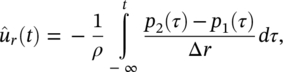

where p₁ and p₂ are the sound pressure signals from the two microphones, ∆r is the microphone separation distance, and τ is a dummy time variable. The caret indicates the finite difference estimate obtained from the “two‐microphone approach.” The sound pressure at the center of the probe is estimated as

(8.36)

and the time‐averaged intensity component in the axial direction is, from Eqs. (8.3), (8.35), and (8.36),

(8.37)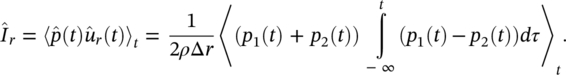

The majority of sound intensity measurement systems in commercial production today are based on the two‐microphone method and the use of condenser microphones, which are the most reliable and stable types available. Some commercial intensity analyzers use Eq. (8.37) to measure the intensity in one‐third‐octave frequency bands. See for example Figure 8.10. Another type of analyzer uses Eq. (8.37) to calculate the intensity from the imaginary part of the cross‐spectrum G₁₂ between the two microphone signals. See for example Figure 8.11.

(8.38)

The time domain formulation and the frequency domain formulation, Eqs. (8.37) and (8.38) respectively, are equivalent. Eq. (8.38), derived originally by Chung [31] for his frequency analysis of engine noise in the mid 1970s, makes it possible to determine sound intensity spectra with a dual‐channel Fast Fourier Transform (FFT) analyzer. Fahy [32] published the same intensity expression in his Letter to the Editor in JASA.

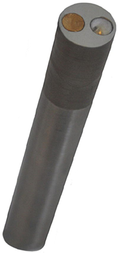
Figure 8.12 shows two of the most common microphone arrangements, “side‐by‐side” and “face‐to‐face” [44]. The side‐by‐side arrangement has the advantage that the diaphragms of the microphones can be placed very near a radiating surface, but has the disadvantage that the microphones shield each other. At high frequencies the face‐to‐face configuration with a solid spacer between the microphones is normally the superior arrangement [44, 45]. Figure 8.13 shows a sound intensity probe with two microphones in the face‐to‐face configuration (Bruel & Kjaer, Denmark.) Figure 8.14 shows two examples of commercial three‐dimensional sound intensity probes.

a) Errors and Limitations in p–p Measurements of Sound Intensity

There are many sources of error in the measurement of sound intensity with two microphones, and a considerable part of the sound intensity literature has been concerned with identifying and studying such errors, some of which are fundamental and others, which are associated with technical deficiencies [37, 44–47]. One complication is that the accuracy depends very much on the sound field under study; under certain conditions even minute imperfections in the measuring equipment will have a significant influence. Another complication is that small local errors are sometimes magnified into large global errors when the intensity is integrated over a closed surface [48].

The following is an overview of some of the sources of error in the measurement of sound intensity. A more detailed discussion is given in Ref. [49]. Those who make sound intensity measurements should be aware of the limitations imposed by:

• The finite difference error [50]
• Errors due to scattering and diffraction [45]
• Instrumentation phase mismatch [47].

Other possible sources of error that are usually less serious are:

• Random errors associated with a given finite averaging time [46] and
• Bias errors caused by turbulent airflow [51].

Chung and Pope demonstrated that a two‐microphone system (in a side‐by‐side arrangement) using the cross‐spectrum formula (Eq. (8.38)) along with microphone switching could measure the sound intensity [52]. This was proved experimentally by confirming that at 1 m from a loudspeaker the intensity measurements gave the same result as that made with single microphones assuming the sound intensity I = p²_rms/ρc. See Figure 8.15a. Later Blaser and Chung [53] compared the sound power propagating along a tube (measured by two microphones) from a loudspeaker source with the sound power radiated out of the tube through a control surface with the two microphone arrangement with the same microphone separation (see Figure 8.15b). By summing the space–time average of the sound intensity measured normal to the control surface (after multiplying by appropriate control area segments) they obtained almost perfect agreement with the in‐duct sound power measurements.

After obtaining sound power estimates of sources by making fixed point measurements, Chung went on to demonstrate that continuously scanning the two side‐by‐side microphone arrangement over a conformal surface around a diesel engine could be used to measure its sound power [19]. Soon after Reinhart and Crocker showed that scanning intensity measurements made on selected parts of a diesel engine gave more accurate results than sound power single microphone measurements on a spherical surface obtained by selective lead wrapping [20].

b) Errors Due to the Finite Difference Approximation

One of the obvious limitations of the measurement principle based on the use of two pressure microphones is the frequency range [25–27, 30]. The finite difference estimate given by Eq. (8.37) is accurate only if the distance between the microphones is much less than the wavelength, as suggested in Figure 8.16; and this clearly implies an upper frequency limit that is inversely proportional to the distance between the microphones. The finite difference error, that is the ratio of the measured intensity  to the true intensity I_r, can be shown to be

(8.39)

for an ideal intensity probe in a plane wave of axial incidence. This relation is shown in Figure 8.17 for different values of the microphone separation distance. Although the finite difference error in principle depends on the sound field [37, 44], the upper frequency limit of intensity probes had generally been considered to be the frequency at which the error given by Eq. (8.36) is acceptably small. Note, however, that the interference of the microphones on the sound field had been ignored. A numerical and experimental study of such interference effects has now shown that the upper frequency limit of an intensity probe with the microphones in the usual face‐to‐face configuration is an octave above the limit determined by the finite difference error if the length of the spacer between the microphones equals the diameter. This is because the resonance of the cavities in front of the microphones gives rise to a pressure increase that to some extent compensates for the finite difference error [45]. See Figure 8.18.

Figure 8.19, which corresponds to Figure 8.17, shows the error calculated for a probe with two half‐inch microphones. It is apparent that the optimum length of the spacer is about 12 mm and that a probe with this geometry performs very well up to 10 kHz [45].

c) Errors in p–p Probe due to Instrumentation Phase Mismatch

Phase mismatch between the two measurement channels is the most serious source of error in the measurement of sound intensity. In the first ground breaking measurements of sound intensity made by Chung and his colleagues in the late 1970s and early 1980s, commercial sound intensity probes with phase‐matched microphones were not available. So they used a pair of high‐quality microphones, cartridges, and preamplifiers in a side‐by‐side configuration. This arrangement has the advantage that the phase mismatch between the two measurement systems can be measured and corrected. The side‐by‐side arrangement of the microphone pair (probe) also allows it to be located closer to noise sources than sound intensity probes now commercially available, which mostly have asymmetric arrangements.

Chung [55] and Chung and Blaser [54] have described three main approaches to make phase‐mismatch corrections as follows. Krishnappa has also described another similar method [58].

1. Transfer Function Approach

This procedure is presented in detail by Chung and Blaser, and Chung [54, 55]. The calibration transfer function (magnitude and phase difference) between the two systems is normally achieved by mounting the two microphones in a circular plate attached to the one end of a circular tube. The two microphones are subjected to the same broadband frequency sound field produced by a loudspeaker mounted at the other end of the tube.

The transfer function thus measured with an FFT analyzer represents the phase and gain difference between the two measurement systems. If the first microphone (#1) is used as a reference, the phase and gain correction [G₁₂]_calibrated is given by:

(8.40)

where H₁₂ is the calibration transfer function and |H₁| is the gain factor of the microphone system #1.

• 2) Microphone Switching Approach

Chung describes the switching procedure as follows, where the intensity in the x‐direction, I_x (ω) is given by:

(8.41)

and where G₁₂ ^S is the cross‐spectrum measured with the two microphone sensing locations interchanged and | H₁| and |H₂| are the gain factors of each microphone. It is seen from Eq. (8.41) above that the phase‐corrected cross spectrum is obtained from the geometric mean of the original cross‐spectrum G₁₂ and the switched cross‐spectrum G₁₂ ^S, or

(8.42)

• 3) Modified Microphone Switching Approach

The modified switching approach has been described and used by Chung and Blaser [54] and Chung [55]. In this approach, the relative phase between the two microphone systems and the gain factors of each system are obtained by taking the square root of the ratio of the original and switched transfer functions. Any broadband signal can be used in determining the transfer functions and the microphones need not be subjected to the same sound fields. The procedure is given by:

(8.43)

where

(8.44)

and where H₁₂ and H₁₂ ^S are the original and switched transfer functions described above.

Chung has discussed the advantages of the three methods described above in Ref. [55] to correct for phase mismatch. In the first method, the Transfer Function Approach, a very sophisticated spectrum analyzer is not needed. It is not necessary to repeat measurements with suitable microphones to take the square root of the complex variable in Eq. (8.42). However, it is usually difficult to measure the transfer function, H₁₂ over a broad frequency range. Less error is likely with use of the second method, the Microphone Switching Approach, with microphones in the side‐by‐side arrangement. However, some intensity probes are not symmetrical and this method cannot be used. The third method is a compromise between the first two methods. A good free field condition is not needed and it saves ensemble‐averaging time. But it is necessary to take the square root of a complex variable.

Some continue to make phase mismatch corrections in intensity measurements, as explained by Chung, to obviate the need to purchase special probes produced by manufacturers and their associated software. However, many now make use of commercial sound intensity probes. In such commercial probes, microphones, and associated electronics are chosen individually in which the phase mismatch has been carefully minimized. In 1987, a special calibrator was produced by Bruel & Kjaer for the calibration of p–p probes. This calibrator makes it possible to simulate an acoustic field of known intensity by positioning acoustical elements between the microphones thus creating a certain frequency‐dependent phase difference between them. The calibrator can then be used to perform particle and sound intensity calibrations of the probe.

Even with the best equipment that is available today, phase mismatch remains a problem. It can be shown that the estimated intensity, subject to a phase error φ_e, is a very good approximation to the true intensity I_r, (which is unaffected by phase mismatch) and it can be written as [59]

(8.45)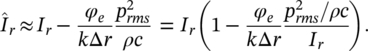

That is, the phase error causes a bias error in the measured intensity that is proportional to the phase error and to the mean square pressure, but inversely proportional to the wave number (and thus frequency) [30, 57].

For a given phase error, φ_e, the bias error in the intensity is proportional to the ratio of the mean square sound pressure to the sound intensity; but it is inversely proportional to the frequency and the microphone separation distance. Ideally the phase error should be zero, of course. In practice one must, even with state‐of‐the‐art equipment, allow for phase errors ranging from about 0.05° at 100 Hz to 2° at 10 kHz. Both the IEC standard and the North American ANSI standards on instruments for the measurement of sound intensity specify performance evaluation tests that ensure that the phase error is within certain limits. Figure 8.20 [60] shows the error in intensity level as a function of frequency for a phase error of 0.3°.

Eq. (8.45) is often written

(8.46)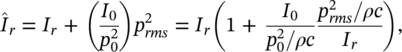

where the residual intensity I₀

(8.47)

has been introduced. The residual intensity, which is normally measured in one‐third octave bands, is the “false” sound intensity indicated by the instrument when the two microphones are exposed to the same pressure p₀. Under such conditions the true intensity is zero and the indicated intensity I₀ should be made very small. A commercial instrument for measuring I₀ in which the two microphones are subjected to the same sound pressure p₀ is shown in Figure 8.21.

The right‐hand side of Eq. (8.46) shows how the error caused by phase mismatch depends on the ratio of the mean square pressure to the intensity in the sound field, which is governed by the conditions in the sound field.

EXAMPLE 8.3

A two‐microphone sound intensity probe has a total phase mismatch of 1° at 400 Hz and the distance between the microphones is 12 mm. The probe measures a sound intensity level of 76.5 dB in a 400 Hz progressive plane wave. What is the true value of the sound intensity level?

SOLUTION

If a phase mismatch φ_e = 1° = π/180 rad exists between the two measuring channels, we determine the approximation error in a plane sinusoidal wave using Eq. (8.39): ε = Î/I = sin(kΔr ± φ_e)/kΔr. Since kΔr = (2πf/c) Δr = 2π(400)(12 × 10⁻³)/344 = 0.0279π. Thus, the underestimation is ε = sin(0.0279π − π/180)/0.0279π = 0.8, so L_ε = 10log(0.8) = −0.97 dB. Now, the overestimation is ε = sin(0.0279π + π/180)/0.0279π = 1.197, and L_ε = 10log(1.197) = +0.78 dB. Therefore, the true intensity will be 76.5 + 0.78 ≈ 75.7 dB or 76.5 − 0.97 ≈ 75.5 dB.

EXAMPLE 8.4

The two microphones in a sound intensity probe are known to have a response phase difference of 0.3° at 63 Hz when the probe is oriented in the direction of propagation of a plane wave. Determine the separation between the microphones such that the maximum approximation error at 63 Hz is −2 dB.

SOLUTION

Since L_ε = 10logε, then ε = 10^−2/10 = 0.63. Now, k = (2πf/c) = 2π(63)/344 = 0.367π, and φ = 0.3^ο = 1.7π × 10⁻³. If kΔr − φ is small, then ε = 1 − (φ/kΔr). Thus, 1 − (1.7π × 10⁻³/0.367πΔr) = 0.63. Solving for Δr gives that the separation between the microphones must be 0.0125 m ≈ 12.5 mm (see Figure 8.20).

Phase mismatch in sound intensity probes is usually described in terms of the so‐called pressure‐residual intensity index:

(8.48)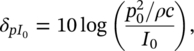

which is a common way of describing the phase error. With a microphone separation distance of 12 mm, the typical phase error corresponds to a pressure‐residual intensity index of 18 dB over most of the frequency range. Figure 8.21 shows a commercial coupler for the measurement of the pressure‐residual intensity index. The error due to phase mismatch is small, provided that the measured pressure‐intensity index δ_pI is much less than the pressure‐residual intensity index (Eq. (8.48)); that is

(8.49)

where

(8.50)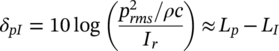

is the pressure‐intensity index of the measurement. The inequality Eq. (8.49) shows that the phase error in the equipment must be much smaller that the phase angle between the two sound pressure signals in the sound field for measurement errors to be minimized. A more specific requirement is given by

(8.51)

where the quantity

(8.52)

is called the dynamic capability index of the instrument and K is the bias error index. The dynamic capability index states the maximum acceptable value of the pressure‐intensity index of the measurement for a given grade of accuracy and is used in the ISO standards. The larger the value of K the smaller is the dynamic capability index, the stronger and more restrictive is the requirement, and the smaller is the error. The condition expressed by the inequality Eq. (8.51) and a bias error index of 7 dB guarantee that the error due to phase mismatch is less than 1 dB. This corresponds to the phase error of the equipment being five times less than the actual phase angle in the sound field. Figure 8.22 gives a plot of the maximum error due to phase mismatch as a function of the bias error index K.

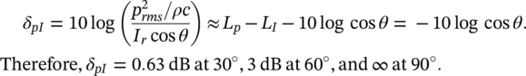
EXAMPLE 8.5

Calculate the pressure‐intensity index in a plane traveling wave field with the intensity probe axis at 30°, 60°, and 90° to the direction of propagation.

SOLUTION

If a plane sound wave is incident at an angle θ to the probe axis, the measured intensity is reduced by a cos θ factor, such that I(θ) = I_r cos θ. Then, in Eq. (8.50) we obtain that

Sound power measurements using sound intensity involve integrating the normal component of the intensity over a surface. The global version of Eq. (8.46) has the form [30, 57]

(8.53)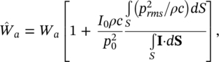

which shows that the global version of the inequality Eq. (8.51) can be written as

(8.54)

where

(8.55)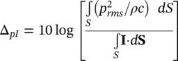

is the global pressure‐intensity index of the measurement. This quantity plays the same role in scanning sound power estimation as the pressure‐intensity index does in measurements at discrete points.

It is obvious that the presence of noise sources outside the measurement surface increases the mean square pressure on the surface, and thus the influence of a given phase error; therefore, phase mismatch limits the range of measurement. Most modern sound intensity analyzers can determine the global pressure‐intensity index concurrently with the actual measurement. Figure 8.23 shows examples of the index measured under various conditions [59]. In practice one should examine whether the inequality Eq. (8.54) is or is not satisfied if there is significant noise from extraneous sources. If the inequality is not satisfied, it can be recommended to use a measurement surface somewhat closer to the source than is advisable in more favorable circumstances. It may also be necessary to modify the measurement conditions – to shield the measurement surface from strong extraneous sources, for example, or to increase the sound absorption present in the room.

d) Calibration of p–p Sound Intensity Probes

Several calibration procedures are required for p–p sound intensity probes in order to ensure accurate measurements are made. The two microphones should be calibrated with a pistonphone as usual. In addition, the IEC standard and the ANSI counterpart standard specify minimum acceptable values of the pressure‐residual intensity index for the probe and the processor system. The test to ensure these minimum values are achieved involves exposing the two microphones to the same sound pressure in a small cavity driven by a broadband noise source. A similar test is carried out on the processor by feeding the same signal to the two channels. As already discussed, the measured pressure‐intensity index, which is equal to the pressure‐residual intensity index, reveals how well the microphones are matched. According to the results of the test, the probe and its associated system are classified as “class 1” or “class 2.”

The pressure and intensity response of the probe should also be checked in a plane propagating wave as a function of frequency. In addition, tests should be performed to ensure that the directional response of the probe follows the ideal cosine law within a specific tolerance. A final test is required for the frequency range below 400 Hz. In this test the intensity probe is exposed to a sound field in a standing wave tube with a prescribed standing wave ratio (24 dB for class 1 probes.) The sound intensity indicated by the system, when the probe is traversed through the resulting interference field, should be within a given tolerance. More details are given by Jacobsen in Refs. [30, 57].

The Bruel and Kjaer Company produces an intensity probe with the microphones arranged in a face‐to‐face arrangement. The probe when it is supplied has microphones which have been specially selected to have an identical phase performance and effective microphone separation. See Figure 8.24. Bruel and Kjaer also produces three calibrators which can be used in the field and laboratory. See Figure 8.25. The checks to the sound intensity system can be finished using these calibrators and checked using the knowledge that the known sound power source shall be accurately determined in a free field (Figures 8.29 and 8.30).

Calibration of a sound intensity system using a p–p intensity probe requires knowledge of:

• Sound pressure transducer properties
  • Sensitivity and gain adjustment
  • Phase matching
  • Effective microphone acoustical separation
• Density of fluid medium
  • Composition of
  • Temperature
  • Ambient pressure

Using the three calibrators in Figure 8.25, the system can be calibrated as follows:

1. The sensitivity and gain can be checked using the B&K 3541 calibrator, see for example Figure 8.26.
2. The manufacturer’s phase matching can be checked using the B&K Type 4297 calibrator (see Figure 8.27) or the B&K Type 3541 calibrator (see Figure 8.28), in which an intensity coupler is used to simulate the microphone separation.

Finally, the sound intensity level is determined in a free field with an omnidirectional sound source and the sound power level in checked and compared with that of a standard sound power level source (Figure 8.29). Also checked are the consistency of the sound pressure, sound intensity and velocity levels (Figure 8.30).

8.6.2 The p–u Method

The p–u method of measuring sound intensity requires the use of two completely different transducers, one to measure the sound pressure and the other the particle velocity. As discussed before, Clapp and Firestone in 1941, Baker in 1955, Burger et al. in 1973, and Van Zyl and Anderson in 1975 all used such devices [12–14, 17, 18]. Unfortunately, all of these devices produced unsatisfactory results.

a) The p–u Measurement Principle

In 1984, Norwegian Electronics manufactured a sound intensity probe, which used a microphone in conjunction with a special transducer [63]. The transducer detected the particle velocity based on the displacement of an ultrasound beam. Unfortunately, the device proved to be difficult to calibrate and was rather bulky and was withdrawn from sale after 10 years in the mid‐1990s [23].

A new miniaturized sensor device known as a Microflown became available for the measurement of particle velocity in the late 1990s [29, 64, 65]. Subsequently this device, when combined with a small microphone, has become available as a small sound intensity probe. The particle velocity sensor is similar to the hot‐wire anemometer employed in the sound intensity probe described by Baker in 1955 [14]. But it is much smaller and does not use wires. Instead two miniature sensors made of silicon nitride on a thin platinum layer are arranged in parallel. They are heated by an electrical current of 10 mA to about 200 °C and sense the fluctuating particle velocity through a cooling effect and related electrical resistance fluctuations. The second sensor is shielded by the first sensor making the intensity device exhibit a cosine directivity in the same way as a p–p probe. Since the sensors are so small (only 1 mm in length) and situated only 40 μm apart, phase shift errors caused by the small spacing can be neglected even at very high frequency. This device is manufactured by Microflown Technologies and probes made for the measurement of intensity in one, two, and three dimensions are available [29, 64–66].

The instantaneous sound intensity is, as before, the product of the sound pressure and particle velocity

(8.56)

and for the simple harmonic case, using complex notation (see Eq. (8.7))

(8.57)

Thus, in the frequency domain

(8.58)

(8.59)

where P(ω) and U(ω) are the Fourier transforms of the sound pressure and particle velocity, and G_pu is the cross spectrum between sound pressure and particle velocity.

The frequency response of the Microflown probe has been found to be relatively flat up to 1 kHz. Then between 1 kHz and about 10 kHz, the frequency response decreases.

b) Sources of Error in p–u Measurement Probes

Some of the sources of error in p–u measurement probes are similar to those in p–p probes and some are different. Phase mismatch is still a problem with p–u systems. With the Microflown probe, phase mismatch in the particle velocity sensor itself is not a problem, but it remains as a problem between the microphone and the sensor. Phase mismatch between the p and u transducers must be corrected otherwise the measurements will be in error. The error is most important in measurements close to a source. This can be illustrated as follows. From

(8.60)

it can be seen that for simple harmonic progressive plane waves when the sound pressure and particle velocity are in phase, φ_r = 0 and cos φ_r = 1 and small phase mismatch errors will have a negligible effect since cos φ_r ≈ 1 until the phase angle becomes very large. However, when the sound pressure and particle velocity are nearly out of phase (for example near a source or a hard reflective surface), then φ_r ≈ 90°, and the reactive intensity becomes

(8.61)

and even a small mismatch error in the estimation of φ_r will have a large effect on the value of I_r measured. See Figure 8.31.

Using complex notation, it can be seen that by introducing a small mismatch error, in φ_r into Eq. (8.57), that the measured time‐average intensity I_r is

(8.62)

when φ_r is small and where I_r is the real intensity and J_r is the reactive intensity. Eq. (8.62) again clearly shows that a small phase error can lead to a significant error in the measured intensity I_r when the time‐average imaginary intensity is much greater than the real intensity J_r >> I_r (e.g. near to a source). However, when the real intensity is much greater than the imaginary intensity I_r >> J_r, then a much greater phase error can be tolerated.

EXAMPLE 8.6

A p–u intensity probe is used to measure a field angle between pressure and particle velocity of 70°. Calculate the maximum instrumentation phase mismatch of the probe to have a systematic error of 1 dB.

SOLUTION

The estimated sound intensity is Î = ½ pu_r cos(ϕ_f ± ϕ_e) and the true intensity is

I = ½ pu_r cos(ϕ_f), where ϕ_f is the angle between the sound pressure and particle velocity and ϕ_e is the phase error. Therefore, the error is 10log (Î/I) = 10log[cos(ϕ_f ± ϕ_e)/cos(ϕ_f)] = 10log[cos(ϕ_e) ∓ tan(ϕ_f) sin(ϕ_e)]. When ϕ_e << 1, the error can be written as 10log[1∓ϕ_e tan(ϕ_f)]. For an error of 1 dB and ϕ_f = 70°, we obtain that ∓ϕ_e tan(70°) = 10^0.1 − 1. Therefore, ϕ_e = ±0.0942 rad ≈ ±5.4° (see Figure 8.31).

c) Calibration of p–u Measurement Probes

Unfortunately, p–u intensity probes are unlike p–p probes, in which phase mismatch can be corrected in principle by reversing the probe in the sound field. This is because the phase mismatch in this case with a p–u probe does not change sign with probe reversal and thus cannot be canceled out.

Fahy has discussed the importance of correcting for p–u phase mismatch in reference [24]. Unfortunately, currently there are no standardized methods for calibrating p–u probes or for determining and correcting for phase mismatch. A small p–u probe was brought into production about 1990 (see Figure 8.32). The Microflown p–u probe, since it is much smaller, can be put in a standing wave tube. According to the Microflown company their probe can be calibrated in a standing wave tube in the frequency range 20 Hz–3.5 kHz. At the end of the tube, the phase shift between sound pressure and particle velocity should be equal to ±90°. Near to the end of a rigidly terminated standing wave tube the phase shift is a simple sine function.

Jacobsen et al. [67, 68] have also investigated the calibration of this p–u probe using two other approaches. One calibration method is known as the “Piston on a Sphere” and is used in the frequency range 10–400 Hz. The other method requires the use of a special loudspeaker with a known acoustical calibration and a reference microphone placed in an anechoic room. This method is useful in the range 300 Hz–20 kHz. Since the calibration of the Microflown probe is complicated, most users will need to rely on that carried out by the manufacturer [68]. The Microflown probe has now been used to make sound power measurements on large machines [69]. Its uses in scanning and measurement criteria have also been discussed [70, 71].

8.6.3 The Surface Intensity Method

With the surface intensity method, in principle the surface vibration velocity can be measured with a noncontacting device, such as a laser Doppler system, or a contacting device such as an accelerometer. The sound pressure still has to be measured with a microphone.

The disadvantage of this method is that it is laborious. The surface velocity must be measured at numerous locations and the sound pressure must also be sensed close to these locations in which the sound field is normally quite reactive. However, the method does have the advantage that the information about the surface vibration can be also of considerable value independently and allows the radiation efficiency of the surface to be calculated as part of the measurement process. In addition, the microphone measurements must be made in the near field and although this has measurement difficulties, background noise is less of a problem because the source sound is normally dominant. Most attention to date has been given to the p–p and p–u approaches described in Sections 8.6.1 and 8.6.2 above.

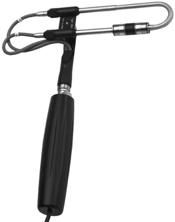
The surface intensity technique which uses an accelerometer mounted on a vibrating surface and a microphone located close to the accelerometer has been under development since about 1974. Macadam described the use of this technique in the measurement of the sound power radiated from room surfaces in lightweight buildings [72, 73]. Hodgson also discussed this technique and its use on a large centrifugal chiller machine [74]. Brito investigated theoretically and experimentally the case of a vibrating rectangular flexible panel and obtained good agreement [75, 76]. Kaemmer and Crocker [77–79] measured the sound power of a vibrating cylinder using the surface intensity method and compared it with the reverberation room method and theory. McGary and Crocker continued development of the surface intensity technique [80–83]. They then applied it successfully to the determination of the sound intensity radiated from the different surfaces of a Cummins NTC 350 (260 kW) diesel engine [80–82]. They obtained good results when they carefully accounted for phase shifts between the microphone and accelerometer signals [83]. Although, the surface intensity probe is more complicated and more difficult to calibrate than a sound intensity probe, it is still used by some. See for example the hand‐held probe developed by Hirao et al. and shown in Figure 8.33 [84].

a) The Surface Intensity Principle

In the case of surface intensity measurements, the velocity u_n normal to the vibrating surface areas S can be found directly by various noncontacting devices or by integrating the signal from a surface‐mounted accelerometer. The pressure p can be measured by a microphone located close to the accelerometer. The finite distance between the noncontacting device or accelerometer and the microphone introduces a time delay Δt between pressure and velocity signals. This can be approximately related to a phase shift ϕ by Δt = ϕ/2πf where f is the frequency (Hz). As with the p–u method, the intensity is usually computed in the frequency domain by feeding the velocity and pressure signals into an FFT analyzer, since the spectral distribution of sound power is usually required. The sound intensity may be shown to be [77, 78]

(8.63)

where C_up is the co‐spectrum (real part) and Q_up is the quad‐spectrum (imaginary part) of the one‐sided cross‐spectral density between velocity and pressure G_up:

(8.64)

b) Sources of Error in Surface Intensity Measurements

The phase shift between the surface velocity and the sound pressure must be corrected otherwise large errors will occur. The phase shift can be caused by the finite distance between the microphone and the vibrating surface. This can be approximated by the travel time in a progressive wave (see Figure 8.34). However, a phase error can also be caused by the velocity and pressure instrumentation. The total error E in intensity caused by uncorrected phase shift can be written as [78]

(8.65)

The effect on the estimate of the intensity of undetected phase errors is seen to be a function of ϕ and also the ratio of the quad‐to co‐spectrum (imaginary to real part of the cross‐spectrum). The effect of the ratio Q_up /C_up and uncorrected phase shift ϕ on the intensity is seen to be extremely important. If the quad‐spectrum (imaginary part) is much larger than the co‐spectrum (real part), then even moderate uncorrected phase shifts can cause large errors in the sound intensity measurements.

c) Calibration of Surface Intensity Measurement Systems.

It is obvious that it is very important to measure and correct for phase shift caused by the propagation of sound waves from the surface velocity probe or accelerometer to the pressure sensing device. Additional phase shifts between the velocity/accelerometer sensor and the pressure sensor can also be caused by the associated electronics. In their work with accelerometer/pressure measurements (see Figure 8.35) Kaemmer and Crocker, and McGary and Crocker studied this problem [78, 79, 82].

McGary and Crocker measured the phase shift caused by the microphone/accelerometer separation and also the instrumentation.

Noting that G_ap(ω) = −jωG_up(ω), and that G_ap = G*_pa, Eq. (8.65) can be written as

(8.66)

which is plotted in Figure 8.36. It is observed that the error caused by uncorrected phase shifts depends strongly on the ratio of C_pa/Q_pa.