The way in which the brain interprets the neural pulses is still a matter for research. However, various experiments have been conducted on groups of people to determine people’s average sensation of loudness, etc. We should stress that no one’s hearing is exactly the same as any other and hence we must find statistical responses.
Figure 4.6 shows equal loudness contours for pure tone sounds. Note that the lowest curve in Figure 4.6 is labeled MAF (minimum audible field). This is the hearing threshold, the quietest sounds, on average, at any frequency that average young people can hear.
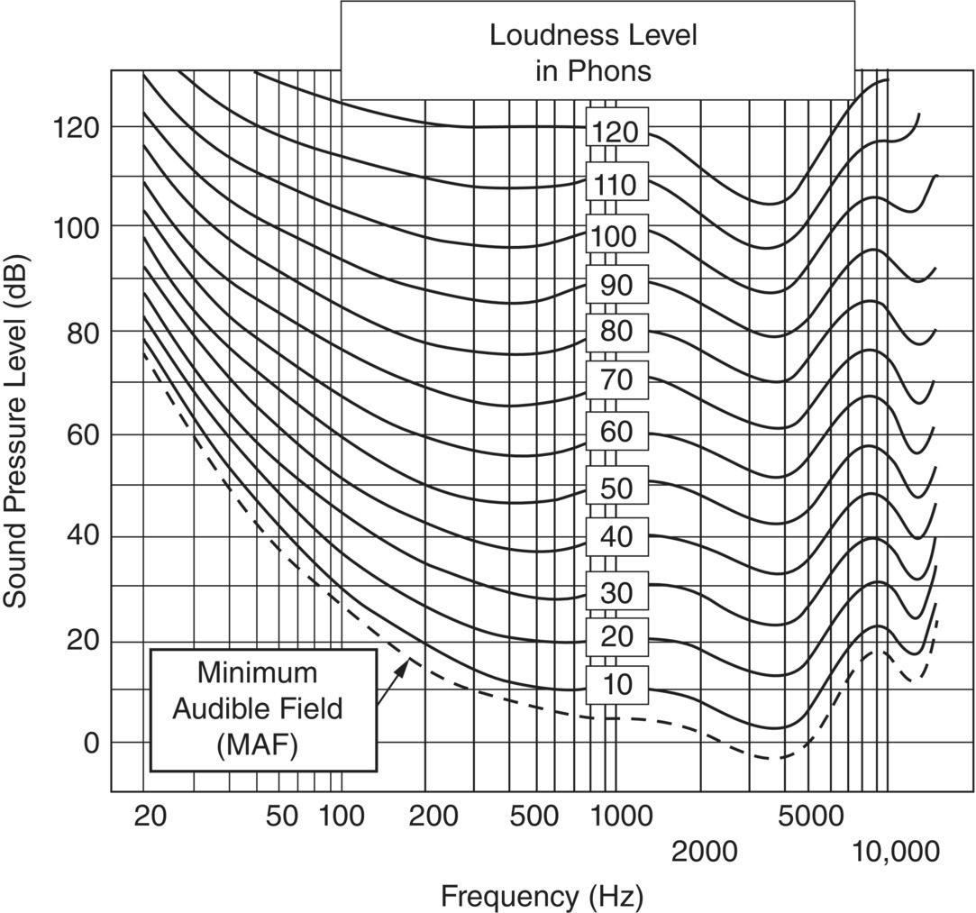
We should note that there are two ways that we can measure the hearing threshold and the equal loudness contours. The first way is to present the listener with a free progressive wave field at a discrete frequency. This is the method which was used to obtain the results in Figure 4.6. Such measurements are normally made with the listener facing the source in an anechoic room where there are no reflections. The second way (which is used more frequently) is to present the listener with sounds played through earphones. There are some small differences in the results obtained by the two methods. The equal loudness contours are determined as follows. For the 60‐phon curve, the listener is first presented with a pure tone at 1000 Hz at a sound pressure level of 60 dB. Then he is presented with a pure tone at, for example, 500 Hz. The pure tones are presented alternately to the listener every few seconds. The level of the 500 Hz tone is adjustable and the listener is asked to adjust the level of the 500 Hz tone until the two tones sound equally as loud. The procedure is repeated with pure tones at other frequencies which are continually adjusted to sound equal in loudness to the 1000 Hz pure tones at 60 dB. The curve drawn through these points (when the result is averaged for a large number of people) is called the 60‐phon equal loudness contour. The 70‐phon contour is obtained by finding the sound pressure level of pure tones which seem equally as loud as 1000 Hz pure tone at 70 dB and so on. Finally, the MAF is the contour joining all pure tones which are just audible. Figure 4.6 was determined for a group of young people with healthy ears in the age group 18–25, each person listening with both ears, facing the source, in a free progressive wave acoustic field.
We see from the equal loudness contours that the ear is most sensitive to sound at about 4000 Hz. This is mainly due to a quarter wavelength resonance in the ear canal at this frequency. The increase in sensitivity at 12 000 Hz is mainly caused by diffraction effects around the head.
The equal loudness contours are not flat as the frequency is changed. Notice at 1000 Hz we can just detect sounds of 4 dB, while at 100 Hz they must be 25 dB. Thus the intensity must be 21 dB higher at 100 Hz than 1000 Hz for us to detect a pure tone. This represents a 100‐fold increase in intensity or a 10‐fold increase in sound pressure amplitude. As the sound pressure level is increased, the equal loudness contours became flatter. A 40 dB tone at 1000 Hz appears equally as loud as a 51 dB tone at 100 Hz, an 11 dB increase. A 70 dB tone at 1000 Hz is as loud as a 75 dB tone at 100 Hz, only a 5 dB increase.
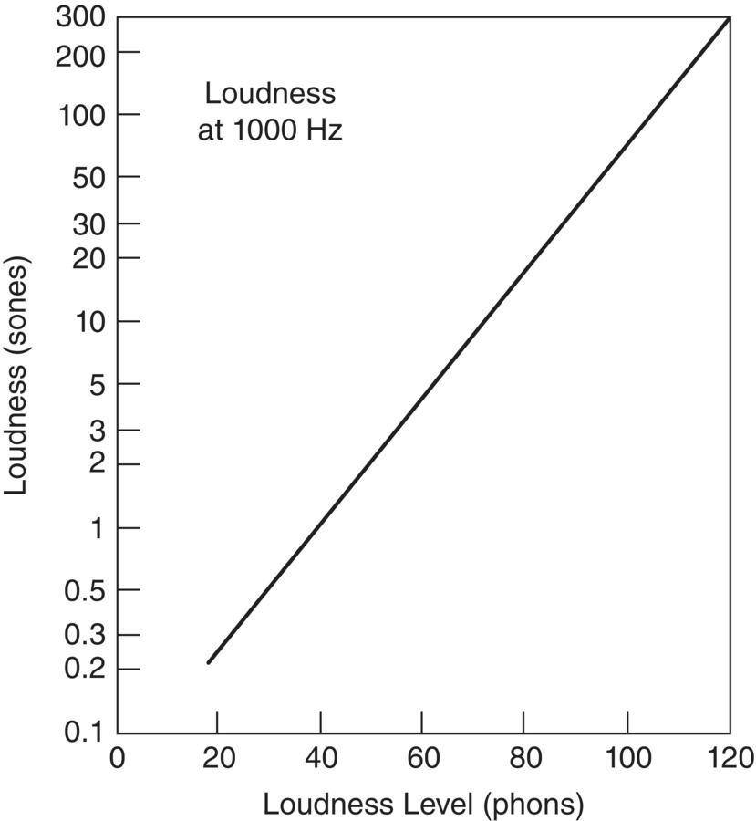
A further experiment has been performed on the loudness of pure tones. This experiment is to determine the increase in sound pressure level for a pure tone apparently to double in loudness. It has been found that for pure tones at 1000 Hz, when the sound pressure level is increased by about 10 dB, the sound appears twice as loud. Fletcher and Munson first commented on this in 1933 [11]. Alternatively we may say that since equal loudness contours join all pure tones with the same loudness levels in phons, then a doubling in loudness occurs when the loudness level increases by 10 phon. This relationship is shown in Figure 4.7 and in the equation
(4.1)![]()
where S is loudness (sone) and P is loudness level (phon).
EXAMPLE 4.1
Equation (4.1) is quite useful since it converts the logarithmic loudness level, phon, into the more useful linear loudness measure, sone. We see from Eq. (4.1) or Figure 4.7 that a loudness level of 40 phons has a loudness of 1 sone, a loudness level of 50 phons has a loudness of 2 sones, and a loudness level of 60 phons has a loudness of 4 sones and so on.
EXAMPLE 4.2
Given three pure tones with the following frequencies and sound pressure levels: 100 Hz at 60 dB, 200 Hz at 70 dB, and 1000 Hz at 80 dB:
- Calculate the total loudness in sones of these three pure tones.
- Find the sound pressure level of a single 2000 Hz pure tone which has the same loudness as all the three pure tones combined.
SOLUTION
- The loudness level in phons of each tone is found from Figure 4.6 and the corresponding loudness in sones is found from Eq. (4.1). Then we have that
- 100 Hz @ 60 dB has P = 50 phons and S = 2 sones200 Hz @ 70 dB has P = 70 phons and S = 8 sones1000 Hz @ 80 dB has P = 80 phons and S = 16 sones
- The total loudness of the combined tones (26 sones) corresponds to a loudness level of P = 10log2(26) + 40. Since log2(26) = ln(26)/ln(2) = 4.7, then P = 87 phons.Now, from Figure 4.6 we observe that a pure tone of 2000 Hz and loudness level of 87 phons has a sound pressure level of 82 dB.
So far we have discussed the loudness of pure tones. However, many of the noises we experience, although they may contain pure tones, are predominantly broadband. Similar loudness rating schemes have been worked out for broadband noise. In 1958–1960, Zwicker [12], taking into account masking effects (see later discussion in Section 4.3.3), devised a graphical method to compute the loudness of a broadband noise. It should be noted that Zwicker’s method can be used both for diffuse and free field conditions and for broadband noise even when pronounced pure tones are present. However, the method is somewhat time‐consuming and involves measuring the area under a curve. It has been well described elsewhere [13].
Stevens [14] at about the same time (1957–1961) developed quite different procedures for calculating loudness. Stevens’ method, which he named Mark VI, is simpler than Zwicker’s method but is only designed to be used for diffuse sound fields and when the spectrum is relatively flat and does not contain any prominent pure tones.
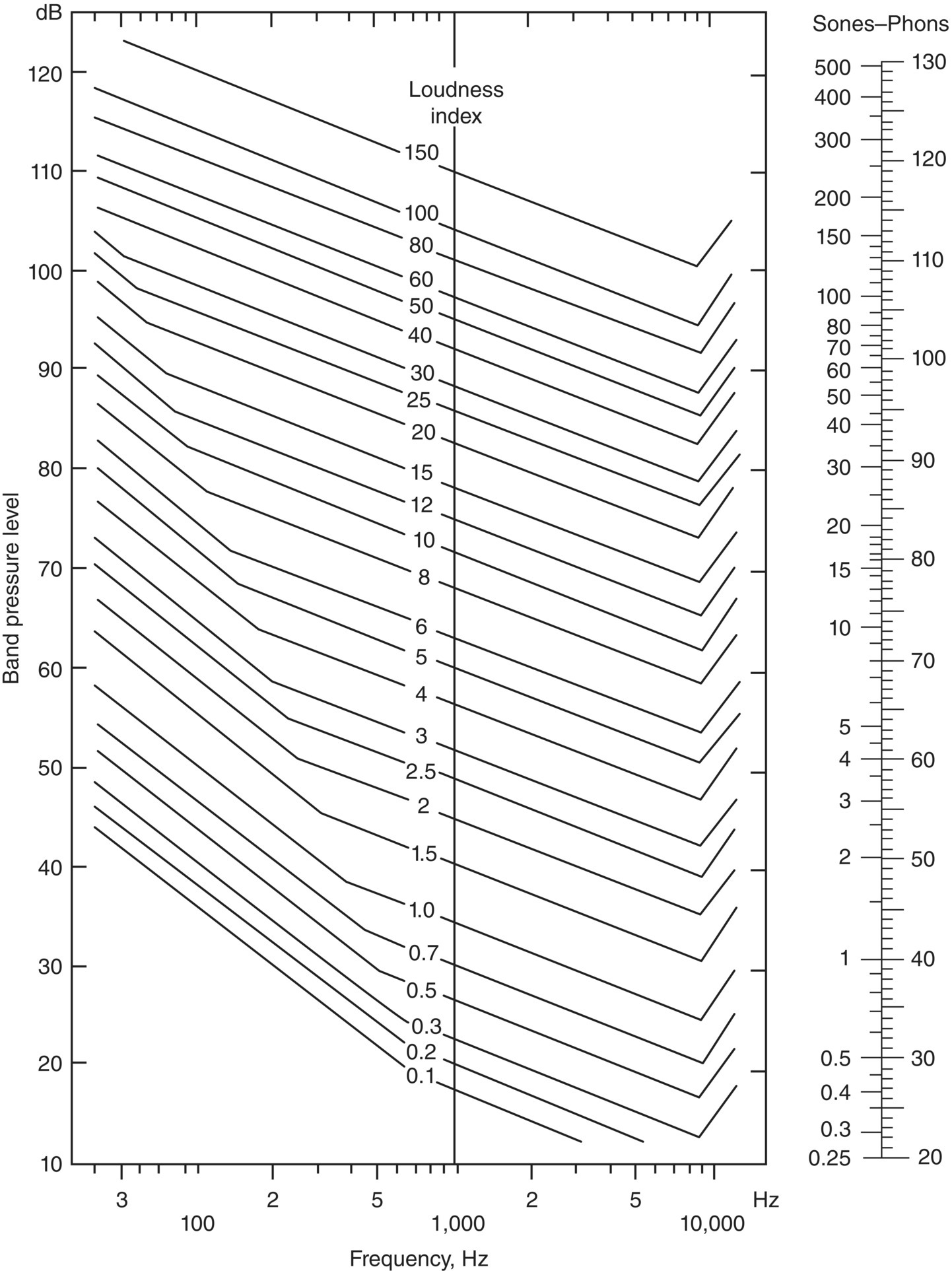
The procedure used in the Stevens Mark VI method is to plot the noise spectrum in either octave or one‐third‐octave bands onto the loudness index contours. The loudness index (in sones) is determined for each octave (or one‐third‐octave) band and the total loudness S is then given by
(4.2)![]()
where Smax is the maximum loudness index and ∑S is the sum of all the loudness indices. The 0.3 constant (used for octave bands) in Eq. (4.2) is replaced by 0.15 for one‐third‐octave bands. The Zwicker method is based on the critical band concept and, although more complicated than the Stevens method, can be used either with diffuse or frontal sound fields. Complete details of the procedures are given in the ISO standard [15] and Kryter [16] has discussed the critical band concept in his book.
EXAMPLE 4.3
The octave band sound pressure levels (see column 2 of Table 4.1) of the noise from machines in a factory are given for the center frequencies (see column 1 of Table 4.1). Calculate the loudness level.
SOLUTION
From Figure 4.8 the loudness indices, S, given in column 3 of Table 4.1 are found.
We obtain that Smax = 26.5 and ∑S = 134.2. Thus from Eq. (4.2) the loudness is: S = 26.5 + 0.3 (134.2 − 26.5) = 59 sones (OD, Octave Diffuse) and from Eq. (4.1), or Figure 4.7, the loudness level is: P = 99 phons (OD).
Table 4.1 Octave band levels of factory noise and Stevens’ loudness indices.
| Octave band center frequency, Hz | Octave band level, dB | Band loudness index S |
|---|---|---|
| 31.5 | 75 | 3.0 |
| 63 | 79 | 6.2 |
| 125 | 82 | 10.5 |
| 250 | 85 | 15.3 |
| 500 | 85 | 18.7 |
| 1000 | 87 | 26.5 |
| 2000 | 82 | 23.0 |
| 4000 | 75 | 17.5 |
| 8000 | 68 | 13.5 |
There are several other aspects of loudness which we have not had room to discuss in this book, e.g. impulsive noise, and monaural and binaural loudness. Readers will find these well covered in Kryter’s book [16].
Leave a Reply