Exhaust System Modeling

It will now be shown that for any linear passive muffler element that the TL is a property only of the muffler geometry (i.e. four‐terminal constants A, B, C, and D) and unaffected by connection of subsequent muffler elements or source or load impedances. On the other hand, it will be shown that the IL is affected by the source and load impedances. Finally, if it is desired to predict the SPL outside of the tail pipe it is necessary to have a knowledge not only of the source impedance and load impedance but also of the source strength – either sound pressure or volume velocity.

The TL of a muffler is the quantity most easily predicted theoretically and is certainly of guidance in muffler design. However, either IL or a prediction of the sound pressure radiated from the tail pipe is much more useful to the muffler designer and these are now discussed.

10.7.1 Transmission Loss

The source‐muffler‐termination system may be modeled as an equivalent electrical circuit [5, 30, 62, 63, 65]. The velocity source model in Figure 10.26b will be used in the derivations of TL (although the pressure source model gives the same result). For simplicity, the mean flow is ignored and the Mach number set to zero, M = 0. The cross‐sectional areas of the muffler inlet and outlet pipes S₀ are assumed to the equal and there is no mean temperature gradient in the muffler system. To determine the TL, the incident and transmitted pressure amplitudes  and  are needed. The transmitted pressure  is most easily determined by making the tail pipe non‐reflecting (Z_r = ρc/S₀). Thus .

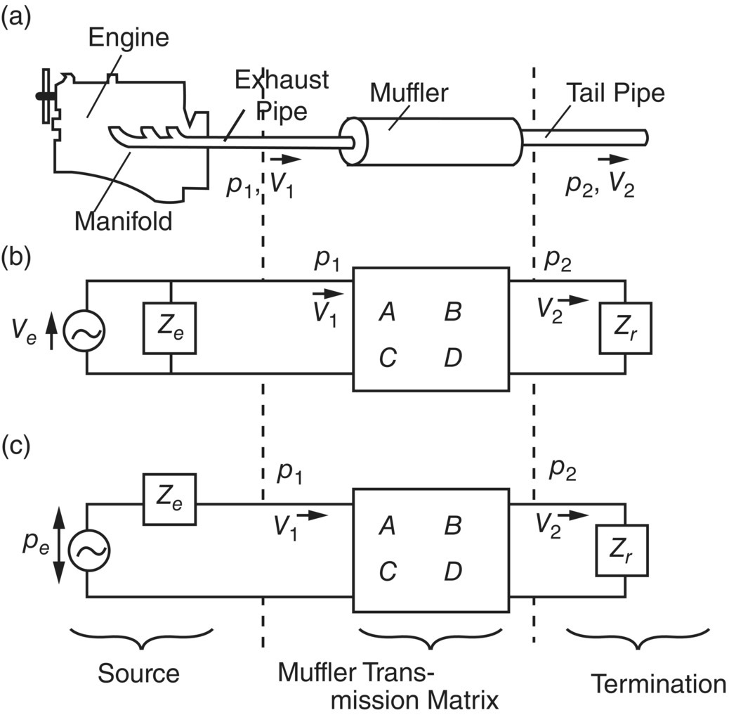
From Figure 10.26b (see Eqs. (10.2a), (10.3a), and (10.3b)):

(10.47)

(10.48)

(10.49)

and from Eqs. (10.38), (10.39) and (10.44):

(10.50)

(10.51)

From the definition in Figure 10.4b:

(10.52)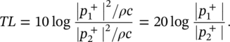

Then eliminating  in Eqs. (10.50) and (10.51) and substituting into Eq. (10.52) gives:

(10.53)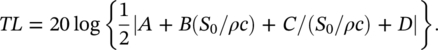

Equation (10.53) is a similar result to that obtained by Young and Crocker [46]. Except note that in Ref. [46] particle velocity was used instead of volume velocity and so A, B, C, and D have slightly different definitions. Sullivan [30] has also derived a result similar to Eq. (10.53) in which the mean temperature, cross‐sectional area and mean flow in pipes l and 2 are different.

The TL is convenient to predict but somewhat inconvenient to determine experimentally. With some care it is possible to construct an anechoic termination from an absorbently‐lined horn or use of absorbent packing [47] enabling  to be measured directly. The quantity  can also be determined when the source (in Figure 10.26) is a loudspeaker, by measuring the standing wave in the exhaust pipe, using a microphone probe tube (although it is a laborious process). The TL can be measured for an absorbent silencer in this way. However, if the TL is determined in the “real‐life” situation with an automobile engine as a source, the microphone probe tube is placed under severe environmental conditions of high temperature and moisture condensation. Alternatively, as suggested by Seybert and Ross, the TL can be measured using two microphones instead of a probe tube [61]. However, if an automobile engine tail pipe anechoic termination is used, it must be of special design to withstand the high temperature. The IL is of much more practical interest and much easier to measure when an engine is a source. It is also easy to measure with absorbent silencers in ducted systems. The measurement of the IL is discussed next.

10.7.2 Insertion Loss

Using Figure 10.26b again gives:

(10.54)

(10.55)

where Z_e and Z_r are the source internal impedance and tail pipe or exhaust duct radiation impedance, respectively. Then from Eq. (10.44):

(10.56)

(10.57)

Substituting for V₁ from Eqs. (10.54) into (10.57) and combining Eqs. (10.56) and (10.57) to eliminate p₁ gives:

(10.58)

If a different muffler with four‐terminal parameters A′, B′, C′, and D′ is now connected to the engine, a new pressure  results:

(10.59)

Thus

(10.60)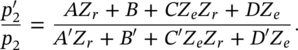

This result is similar to that obtained by Sullivan [30]. If  is measured with no muffler in place and only a short (in wavelengths) exhaust pipe, then A′ = D′ = 1, and B′ = C′ = 0,

(10.61)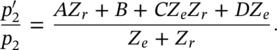

This result is similar to that obtained in Eq. (10.53). Since

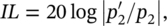
it is seen from either Eqs. (10.60) or (10.61) that unlike the TL, IL depends on both the internal impedance of the source and the tail pipe radiation impedance, besides the transmission characteristics of the muffler itself. Several researchers in the 1970s predicted the IL of mufflers installed on engines, e.g. Young [45] and Davies [66]. However, they have normally had to rely on assumed values of engine impedance (e.g. Z_e = 0, ρc/S_0, etc.), since measured values were not available. Young’s results for IL [45], will be discussed later in Section 10.10.

In prediction of IL, Z_r must also be known. Discussion on the problems of estimating Z_e and Z_r follows in a later section.

If the source and radiation impedances are assumed to be Z_e = Z_r = ρc/S₀, then Eq. (10.61) becomes:

(10.62)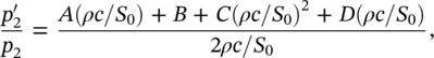

(10.63)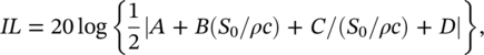

a result identical to Eq. (10.53). This demonstrates the fact that, in the general case, the muffler TL is not equal to the IL except when the IL is measured with source and termination impedances equal to the characteristic acoustic impedance ρc/S₀. The same conclusion can be reached intuitively or theoretically. However, it is more difficult to reach this conclusion by studying traveling wave solutions (transmission line theory) in mufflers and the exhaust and tail pipes than by using the transmission matrix theory.

10.7.3 Sound Pressure Radiated from Tailpipe

A prediction of this quantity is of probably more importance to muffler designers than a knowledge of either TL or IL. After all, the radiated SPL is the quantity which finally determines the acceptability of a muffler. Examining Eq. (10.58), shows that if the source volume velocity source strength V_e, source impedance Z_e, radiation impedance Z_r and muffler four‐terminal (four‐pole) parameters A, B, C, and D are known, then the total sound pressure amplitude (and phase) at the end of the tail pipe p₂ can be calculated. It is a fairly simple matter to calculate the radiated pressure amplitude p_r at distance r from the tail pipe or flow duct outlet [39, 40, 42]. For engine exhaust systems, the method used is to assume monopole radiation from the tail pipe so that the net sound intensity transmitted out of the tail pipe is equal to the intensity in the diverging spherical wave at radius r. This gives:

(10.64)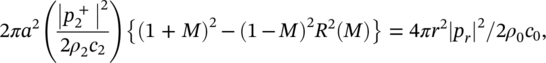

where a is the tail pipe radius and R(M) the tail pipe reflection coefficient (dependent on Mach number M) of the mean flow. Subscript 2 refers to conditions just inside the tail pipe. From Eqs. (10.40) and (10.42), at any station in the muffler:

(10.65)

and at the tail pipe exit:

(10.66)

Thus, at the tail pipe or duct exhaust exit, from Eqs. (10.65) and (10.66):

(10.67)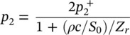

and substituting Eqs. (10.67) into (10.58) gives:

(10.68)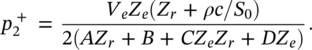

Taking the modulus of Eq. (10.68) and substituting it into Eq. (10.64) eliminates  and gives the pressure |p_r| in terms of the source volume velocity, V_e, the engine and tail pipe radiation impedances, Z_e and Z_r, the muffler four‐pole parameters, the tail pipe reflection coefficient R(M) and the mean‐flow Mach number in the tail pipe, M.