Energy and Power Spectral Densities

In the case of nonperiodic signals (see Section 1.3.2), a quantity called the energy density function or equivalently the energy spectral density, S(f), is defined:

(1.12)

The energy spectral density S(f) is the “energy” of the sound or vibration signal in a bandwidth of 1 Hz. Note that S(ω) = 2πS(f) where S(ω) is the “energy” in a 1 rad/s bandwidth. We use the term “energy” because if x(t) were converted into a voltage signal, S(ω) would have the units of energy if the voltage were applied across a 1 Ω resistor. In the case of the pure tone, if x(t) is assumed to be a voltage, then the mean square value in Eq. (1.8) represents the power in watts.

In the case of random sound or vibration signal we define a power spectral density G_x(f). This may be derived through the filtering – squaring – averaging approach or the finite Fourier transform approach. We will consider both approaches in turn.

Suppose we filter the time signal through a filter of bandwidth Δf, then the mean square value

(1.13)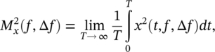

where x(t,f,Δf) is the filtered frequency component of the signal after it is passed through a filter of bandwidth Δf centered on frequency f. In the practical case, the filter bandwidth, Δf, could be, for example, a one‐third octave or smaller. The power spectral density is defined as:

(1.14)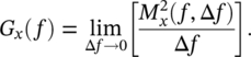

The power spectral density may also be defined via the finite Fourier transform [12, 13]

(1.15)

Note the difference between Eqs. (1.15) and (1.12). We notice that G_x must be a power spectral density because of the division by time. The unit of power spectral density is U²/Hz, where U is the unit of the measured signal. The square root of the power spectral density, often called the rms spectral density, has a unit of . For discussion in greater detail on analysis of random signals the reader is referred to References 1, 2, 7–9. Often in practice we define a new spectral density  which does not contain energy at negative frequencies but only exists in the region 0 < f < ∞. The power spectral density of the random noise in Figure 1.5 is plotted in Figure 1.8.