Bayes’ Theorem – The Forecasting Pillar of Data Science

Are you planning to become a data scientist? If yes, you must read this extensive article on Bayes’ Theorem for Data Science.

No data scientist can work without a complete understanding of conditional probability and Bayesian inference. So, today, we will discuss the same with the help of examples and applications. More importantly, we will discuss how Data Scientist use Bayes’ Theorem.

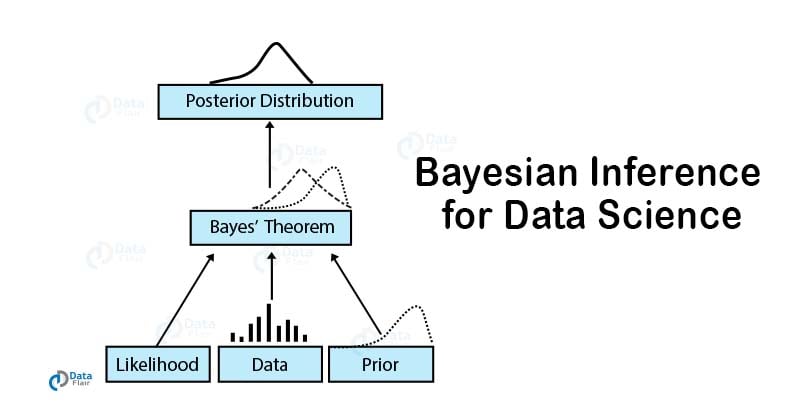
Bayes’ Theorem is the most important concept in Data Science. It is most widely used in Machine Learning as a classifier that makes use of Naive Bayes’ Classifier. It has also emerged as an advanced algorithm for the development of Bayesian Neural Networks.

The applications of Bayes’ Theorem are everywhere in the field of Data Science. Let us first have an overview of what exactly Bayes’ Theorem is.

What is Bayes’ Theorem?

Bayes’ Theorem is the basic foundation of probability. It is the determination of the conditional probability of an event. This conditional probability is known as a hypothesis. This hypothesis is calculated through previous evidence or knowledge.

This conditional probability is the probability of the occurrence of an event, given that some other event has already happened.

The formula of Bayes’ Theorem involves the posterior probability P(H | E) as the product of the probability of hypothesis P(E | H), multiplied by the probability of the hypothesis P(H) and divided by the probability of the evidence P(E).

Let us now understand each term of the Bayes’ Theorem formula in detail –

• P(H | E) – This is referred to as the posterior probability. Posteriori basically means deriving theory out of given evidence. It denotes the conditional probability of H (hypothesis), given the evidence E.
• P(E | H) – This component of our Bayes’ Theorem denotes the likelihood. It is the conditional probability of the occurrence of the evidence, given the hypothesis. It calculates the probability of the evidence, considering that the assumed hypothesis holds true.
• P(H) – This is referred to as the prior probability. It denotes the original probability of the hypothesis H being true before the implementation of Bayes’ Theorem. That is, this probability is without the involvement of the data or the evidence.
• P(E) – This is the probability of the occurrence of evidence regardless of the hypothesis.

Bayes’ Theorem Example

Let us assume a simple example to understand Bayes’ Theorem. Suppose the weather of the day is cloudy. Now, you need to know whether it would rain today, given the cloudiness of the day. Therefore, you are supposed to calculate the probability of rainfall, given the evidence of cloudiness.

That is, P(Rain | Clouds), where finding whether it would rain today is the Hypothesis (H) and Cloudiness is the Evidence (E). This is the posterior probability part of our equation.

Now, suppose we know that 60% of the time, rainfall is caused by cloudy weather. Therefore, we have the probability of it being cloudy, given the rain, that is P(clouds | rain) = P(E | H).

This is the backward probability where, E is the evidence of observing clouds given the probability of the rainfall, which is originally our hypothesis. Now, out of all the days, 75% of the days in a month are cloudy. This is the probability of cloudiness or P(clouds).

Also, since this is a rainy month of the year, it rains usually for 15 days out of 30 days. That is, the probability of hypothesis of rainfall or P(H) is P(Rain) = 15/30 = 0.5 or 50%. Now, let us calculate the probability of it raining, given the cloudy weather.

P(Rain | Cloud) = (P(Cloud | Rain) * P(Rain)) / (P(Cloud))
= (0.6 * 0.5) / (0.75)
= 0.4

Therefore, we find out that there is a 40% chance of rainfall, given the cloudy weather.

After understanding Bayes’ Theorem, let us understand the Naive Bayes’ Theorem. The Naive Bayes’ theorem is an implementation of the standard theorem in the context of machine learning.