Some of the most common practical applications of sound intensity measurements are now discussed. In 1978, Chung and Pope demonstrated that using a two‐microphone probe that sound intensity could be measured both (i) at fixed points in the near field (2.5 cm) from a loudspeaker source and (ii) at 12 points on a hemisphere of 1 m radius surrounding the source [52]. Then using these two measurements and by integration over the hemisphere they obtained sound power level estimates agreeing within 0.4 dB over the frequency range 500–5000 Hz. In 1979, Chung used the scanning procedure to identify parts of a diesel engine [19]. Soon after, Crocker et al. used conformal surface scanning to source‐identify diesel engines [20]. They were able to verify that surface scanning on an engine produced results very similar to those made with fixed points using single microphones and making the far field assumption I = p2/ρc on a spherical array around the engine. They were also able to demonstrate that sound intensity could be used to determine the transmission loss of partitions by surface scanning as accurately as with single microphone measurements using the two‐room method [21, 22].
Sound intensity measurements became widely used in industry in the early 1980s. But a fundamental concern remained whether to measure the intensity at fixed points or to use the faster and more convenient approach of scanning the intensity probe over a control surface encompassing the source. Several researchers conducted theoretical and experimental studies to compare the accuracy of results for the sound power of sources made using sound intensity scans compared with fixed points. In 1984, Bockhoff studied this surface sampling problem using a numerical simulation of continuous scanning (moving the probe over a plane control surface) compared with the use of discrete fixed points measurements on the surface [85]. He concluded that “continuous scanning (even with non‐constant (speed) provides a higher accuracy than fixed point measurements” [85].
In 1986 Pope published theoretical and experimental studies of the sound power of a reference source located over a reflecting surface [86]. The spatial sampling was made on a hemispherical control surface. Pope also concluded that for a “given number of measurements, scan averaging can be expected to yield better sound power estimates than point sampling” [86]. In addition, Crocker raised the issue in 1986 with his editorial “To scan or not to scan” [87]. Yang and Crocker also re‐examined the questions in 1994 with a computer simulation of sound intensity sampling with fixed points and with scanning of a source in the presence of background noise [88]. They similarly concluded that “the scanning method is more accurate that the fixed point method” [88]. Most engineering measurements of sound power and transmission loss of partitions using sound intensity are made with the scanning method. The rest of Section 8.7 reviews a number of practical results.
8.7.1 Sound Power Determination
One important application of sound intensity measurements is the determination of the sound power of operating machinery in situ. Sound power determination using intensity measurements is based on Eq. (8.5), which shows that the sound power of a source is given by the integral of the normal component of the intensity over a surface that encloses the source. Figure 8.37 shows measurements of the normal intensity measured over hemispherical and rectangular surfaces, where the total sound power of a machine source is desired. Theoretical considerations seem to indicate the existence of an optimum measurement surface that minimizes measurement errors. In practice a surface of a simple shape at some distance, approximately 25–50 cm, from the source is recommended by some, as illustrated in Figures 8.38 and 8.39. If there is a strong reverberant field or significant ambient noise from other sources, the measurement surface should be chosen to be somewhat closer to the source under study. Such measurements made closely following the source contour are known as conformal. Sound power measurements using sound intensity were soon put into practice in industry in North America with good results. See, for example, measurements made on earth‐moving equipment in Figure 8.39 [89]. The measurements (which have been A‐weighted) show surprisingly good agreement between the results obtained in three different environments, one of which had high background noise (see Table 8.1). The outdoor free field result was taken as the reference. Figure 8.40 shows sound power measurements made on a reciprocating compressor using sound intensity [90]. Figures 8.41 and 8.42 show sound power measurements made on vehicles using gated sound intensity [91].
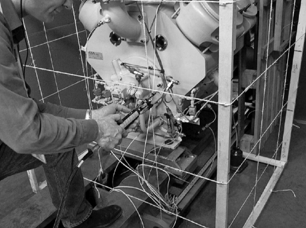
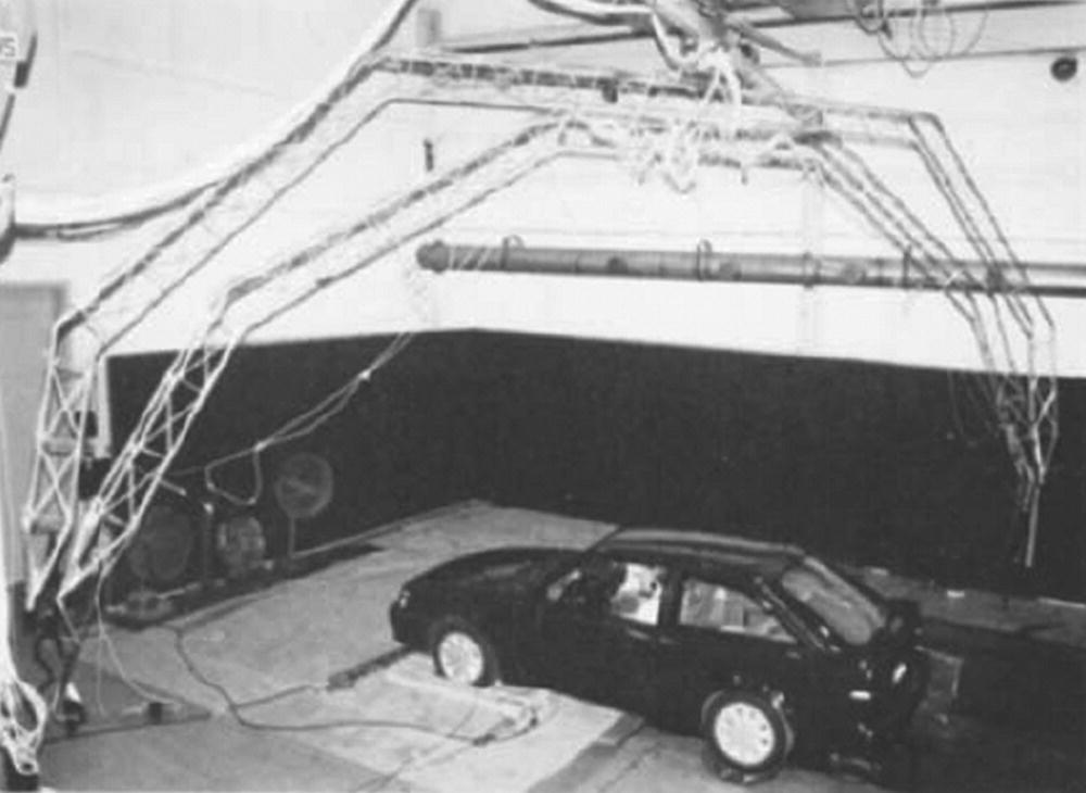
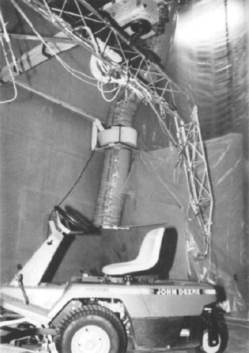
Table 8.1 Sound power measurement by pressure vs. intensity techniques in varying acoustical environments. Identical tests on same crawler tractor [89].
| Environment | A‐weighted difference from true value sound power dB | |
|---|---|---|
| By Intensity | By Pressure/Hemisphere | |
| Outdoor free field | −1.0 | 0a |
| Semi‐anechoic lab | −1.0 | +0.4 |
| Typical service shop | −1.3 | +1.8 |
| Reflective cell | — | +4.2 |
| Reverberant room | −1.7 | +8.2 |
a Assumed as “true value.”
The surface integral can be approximated either by sampling at discrete points or by scanning manually or with a robot over the surface as shown in Figure 8.38. As discussed above, a third approach is to scan the probe over a conformal surface such as closely following the outline of a machine source. This is particularly useful when sound radiation from different parts of a machine must be determined. With the scanning approach, the intensity probe is moved continuously over the measurement surface in such a way that the axis of the probe is always perpendicular to the measurement surface. The scanning procedure, which was introduced in the late 1970s on a purely empirical basis, was regarded by some with much skepticism for more than a decade [57], but is now generally considered to be more accurate and far more convenient than the procedure based on fixed points [57]. A moderate scanning rate, say 0.5 m/s, and a “reasonable” scan line density should be used, say, 5 cm between adjacent lines if the surface is very close to the source, 20 cm if it is farther away.
EXAMPLE 8.7
A sound wave traveling in the direction of the probe axis has an intensity level L1 = (+) 73 dB. Another sound wave travels in the opposite direction with an intensity level L2 = (−) 70 dB. The signs indicate the direction of the intensity. Determine the total sound intensity level measured by the probe when both waves travel simultaneously.
SOLUTION
We must add intensity levels in different directions. We convert the levels back to intensity by I = Iref × 10(L/10). Then, I1 = Iref × 10(73/10) and I2 = Iref × 10(70/10). Now, the total intensity considering the directions is IT = Iref × (107.3 − 107) = 9.953 × 10⁻⁶. Finally, the intensity level is LI = 10 × log (9.953 × 10⁻⁶/10−12) = 70 dB.
EXAMPLE 8.8
A box‐like hypothetical surface of 1 m × 1 m × 0.7 m is constructed around a noisy machine located on a reflective ground to determine its sound power through the scanning procedure. With a suitably long averaging time, a sound intensity probe is swept over each surface. The areas and respective space‐average sound intensity levels on the surfaces are: 82 dB on S1 = 1 m2, 70 dB on S2 = 1 m2, 80 dB on S3 = 0.7 m2, 78 dB on S4 = 0.7 m2, and 81 dB on S5 = 0.7 m2. Calculate the sound power and sound power level of the machine.
SOLUTION
The partial sound powers can be found from each side of the box and added. Thus, the total power is:


8.7.2 Noise Source Identification
This is perhaps the most important application. Every noise reduction project starts with the identification and ranking of noise sources and transmission paths. In one study of diesel engine noise, the whole engine was wrapped in sheet lead. The various parts of the engine were then exposed, one at a time, and the sound power was estimated with single microphones at discrete positions on the assumption that Ir ≈ p2rms/ρc. Sound intensity measurements make it possible to determine the partial sound power contribution of the various components directly.
Plots of the sound intensity measured on a measurement surface near to a machine can be used in locating noise sources. Figure 8.43a shows measurement surfaces near to a vacuum cleaner. Figures 8.43b and 8.43c show a mesh diagram and a contour plot of the normal intensity, and Figure 8.43d gives a vector flow diagram of the intensity.
Magnitude plots using arrows are useful in visualizing sound fields. Figure 8.44 shows the sound intensity measured in the vicinity of a violoncello [92].
8.7.3 Noise Source Identification on a Diesel Engine Using Sound Intensity
In these experiments the sound intensity was assumed to be given by
(8.67)![]()
Corrections for phase shift between the two microphone channels were made using the approach of Krishnappa [58]. The true cross‐spectrum G12 between the microphone signals is related to the measured value ![]() 12 by:
12 by:
(8.68)![]()
where T12 is the transfer function between microphone channel systems 1 and 2 and H2 is the gain of microphone system 2. In principle, this approach has some advantage over the switching technique suggested by Chung [54, 55]. Since switching is eliminated, measurements can be made about twice as fast after the phase shift is determined and stored on the FFT.
In this phase shift determination, the 1/4 in. microphones were mounted at the same longitudinal position at the end of a small tube which was excited by a white noise source from a small loudspeaker. The two microphones were subjected to the same signal to obtain the transfer function T12 below the tube cut off frequency. The gain |H2| was obtained separately by supplying microphone number 2 with a signal from a pistonphone.
If phase‐matched microphones and high‐quality microphone amplifiers are used, the standard deviation of the transfer function measured is often greater than the phase error being measured. In such cases it is not necessary to measure phase mismatch errors. Two microphones were used in a side‐by‐side arrangement for the sound intensity. See Figure 8.12.
The area‐averaging intensity technique was used for the engine measurements, with the hand‐held microphone pair being moved just over the engine surface by hand. An ensemble average was made over one hundred and fifty samples during each intensity measurement. The dynamic range of the intensity measurement system was 40 dB but improvements in the computer programming have extended the dynamic range to 80 dB.
The microphone spacing of 8 mm finally chosen allowed accurate intensity measurements to be obtained in the frequency range from about 200 to 7000 Hz [20, 39, 93].
a) Comparison between Sound Intensity and Lead‐Wrapping Measurements
Using this approach and Eqs. (8.67) and (8.68), Reinhart and Crocker measured the sound power radiated by 103 different sub‐areas on the surface on a Cummins NTC 350 (260 kW) diesel engine. A two‐microphone probe was moved over the surface of the engine to obtain the sound intensity radiated by a particular surface area of the engine. The results from groups of areas were summed together to duplicate the eight major areas used in the lead‐wrapping measurements and five major areas in the surface intensity measurements. The engine was run under the same condition of speed and load so that comparisons could be made between the results. Complete details of the sound intensity engine results and measurements are given in Refs. [20, 39, 93]. Figures 8.45 and 8.46 show the sound power obtained by summing over 25 locations on the oil pan. Figure 8.45 shows narrow‐band results. Figure 8.46 shows the results given in Figure 8.45 summed into one‐third octave bands.
It is interesting to note some peaks in the narrow‐band spectrum in Figure 8.45 which are presumably caused by a forcing frequency being close to a structural resonance frequency. Also of interest is the good agreement between the lead‐wrapping and the sound intensity results in Figure 8.46 for frequencies at and above 325 Hz. This result is similar to that for the oil pan when the lead‐wrapping and the surface intensity results are compared in the later section of this chapter. The results for the other major engine surfaces are given in Refs. [20, 39, 93].
Table 8.2 shows a comparison of the overall sound power levels of the engine obtained from the sound intensity, surface intensity and lead‐wrapping methods [39]. It is seen that the three methods all rank the oil pan as the predominant source. The weaker sources seem to be overestimated by the lead‐wrapping approach [39, 93, 94].
Table 8.2 Comparison of overall sound power levels obtained by the sound intensity, surface intensity, and lead‐wrapping methods [39].
| Engine part | Overall Sound Power Level (dB ref. 1 pW) at 1500 rpm and 540 Nm load | ||
|---|---|---|---|
| Sound intensity | Surface intensity | Lead‐wrapping | |
| Oil pan | 102.7 | 103.3 | 102.6 |
| Exhaust manifold, turbocharger, Cyl. Head, and valve covers | 101.4 | — | 101.6 |
| Aftercooler | 100.8 | 101.9 | 100.6 |
| Engine front | 95.0 | — | 100.0 |
| Oil filter and cooler | 91.1 | 93.4 | 98.1 |
| Left block wall | 97.4 | 94.6 | 97.3 |
| Right block wall | 94.8 | 93.3 | 97.3 |
| Fuel and oil pumps | 91.5 | — | 96.3 |
| Sum of oil pan, aftercooler, oil filter and cooler, block walls | 106.1 | 106.4 | 106.7 |
| Sum of all parts | 108.1 | — | 108.8 |
| Bare engine sound power | — | — | 109.5 |
b) Comparison between Surface Intensity and Lead‐Wrapping Measurements
The sound power radiated from five different surfaces of the engine was measured using the surface intensity technique and compared with the sound power radiated from the same surfaces determined from the lead‐wrapping approach [80–82, 94]. The five parts chosen for surface intensity measurements were: (i) the oil pan, (ii) the aftercooler, (iii) the left block wall, (iv) the right block wall, (v) the oil filter and cooler. The exhaust manifold and cylinder head were not investigated because of the intense heat radiated by these parts. High surface temperatures can make acceleration readings difficult or inaccurate and are somewhat dangerous for investigation when moving the accelerometer from location to location. The front of the engine was not examined either, because pulleys there made it very difficult to mount an accelerometer and locate the microphone. Figures 8.47 and 8.48 show the sound power obtained by summing over 24 locations on the oil pan using Eq. (8.5). Figure 8.49 shows narrow‐band results, while Figure 8.48 shows the narrow‐band sound power results presented in Figure 8.49 summed into one‐third octave bands. The curve with symbols O was obtained from the lead‐wrapping method, while the curve with symbols S was obtained from the surface intensity technique. The results for the other four surfaces examined on the engine are given in Refs. [81, 82, 94]. It is seen in Figure 8.48 that the agreement between the two methods is good except at very low frequency (below 315 Hz). At low frequency the lead becomes “transparent” to sound as already discussed and the surface intensity method is less accurate because of calibration difficulties [82]. The trend for the lead‐wrapping results to be higher than the surface intensity results in the lower frequency region was observed for all the five parts examined and is as expected, since lead‐wrapping fails at low frequency.
c) Radiation Efficiency of Different Engine Surfaces
Many authors have theoretically investigated the sound radiation from vibrating surfaces. Provided the edge conditions are known, the sound radiation can be predicted theoretically for flat beams and plates in different modes of vibration, see Chapters 3 and 12. However, except at or near a resonance frequency, it is difficult experimentally to excite a single mode of vibration and to measure the sound power radiated. In practice many modes of vibration are usually excited simultaneously. It is also much more complicated theoretically to predict the sound radiated from curved vibrating surfaces or where the geometry is complicated or when the edge conditions are not well known.
The sound power Wrad radiated by a vibrating surface of area S is given by:
(8.69)![]()
where ρc is the air characteristic impedance, 〈v2〉 is the space‐average of the mean‐square normal surface velocity, and σrad is the structure radiation efficiency. If a single mode is excited, then the quantities are for that mode. If many modes are excited simultaneously, then Eq. (8.69) still applies, but Wrad and 〈v2〉 are the values for the frequency band under consideration and σrad is a value for the frequency band, averaged over the modes excited. Averaged values of σrad have been calculated theoretically for idealized flat vibrating structures, but are difficult to calculate for curved structures with ill‐defined edge conditions. However, averaged values of σrad may be determined experimentally for complicated structures by measuring Wrad and 〈v2〉.
McGary and Crocker attempted to determine σrad for the five surfaces of the diesel engine under examination by measuring Wrad from the surface intensity method and dividing by 〈v2〉 which is also determined as a by‐product of this approach [39, 80–82]. The results for σrad and for the five surfaces (averaged over one‐third octave bands) are given in Ref. [82]. One typical result for the oil pan is presented in Figure 8.49. At high frequency (above about 1000 Hz) all the surfaces had a radiation efficiency approaching one (as theory should predict).
Such radiation efficiency curves, if they can be accurately predicted or measured, can be very useful in engine design in a number of ways. They enable an experimentalist to determine the sound power radiated by each engine surface, simply by measuring the space‐averaged mean‐square velocity (as a function of frequency) on that surface This can easily be accomplished using an accelerometer rather than making a complicated or sophisticated intensity or sound power measurement. Also, in principle, if theory can be used to predict the vibration of different surfaces of an engine in the design stage, then the sound power radiated by the different surfaces can also be predicted before the engine is constructed.
8.7.4 Measurements of the Transmission Loss of Structures Using Sound Intensity
The transmission loss (sound reduction index) is a measure of the performance of a structure in preventing transmission of sound from one space to another. It is defined as 10 times the logarithm (to base 10) of the ratio of the sound power incident on the dividing structure to the sound power radiated on the receiving side. In principle the receiving space should be anechoic. The evaluation of the transmission loss of panels and partitions is very important in several noise problems, in particular with panels in aircraft, spacecraft, surface vehicles and buildings.
The traditional method of measuring transmission loss requires the use of a very expensive transmission suite consisting of two vibration‐isolated reverberation rooms. The incident sound power is deduced from an estimate of the spatial average of the mean square sound pressure in the source room on the assumption that the sound field is diffuse, and the transmitted sound power is determined from a similar measurement in the receiving room where, in addition, the reverberation time must be determined. In 1980, Crocker was the first to describe a new method for the determination of the transmission loss of panels [21, 22].
This method involves the measurement of the incident and transmitted sound intensities. The incident intensity is determined from measurements of the space‐averaged mean square sound pressure 〈prms2〉 in a reverberation room on the source side of the panel. It was checked to see if the space‐averaged value of 〈prms2〉s/4ρc would be a good estimate of the intensity on the source side of the panel. Figure 8.50 confirms that it is [22]. Here in Figure 8.50, the diffuse field intensity ① is compared with the intensity passing through the open window with the panel absent ②. The transmitted intensity is measured directly, using the two‐microphone technique. One advantage of this sound intensity method is that it uses one reverberation room instead of two as used in the conventional transmission suite method. Another advantage is that it makes possible the identification of the energy transmitted through different parts of composite panels (for example, panels made from a heavy solid wall with lightweight windows) [22]. Measurements of transmission loss made with this method compare favorably with those made using the conventional method and the simple mass law theory [22]. This method has now been standardized. See Section 8.9 and ISO standards 15 186-1 and 15 186‐2 and ASTM standard E 2249‐02 (2009).
It would be attractive to eliminate the use of a reverberation room on the source side of the panel. Unfortunately, this is not normally possible because direct measurements of intensity on the source side give the vector sum of the incident and reflected intensities. What is required on the source side is solely the incident intensity. Ideally the receiving space should be very quiet and non‐reverberant as in the case of an anechoic room. In practice, almost any relatively non‐reverberant environment on the receiving side of the panel is sufficient, provided the background noise levels are steady and low. The transmitted sound intensity is measured directly using a sound intensity probe.
When a reverberation room is available on the source side of a panel, it is normally best to estimate the incident sound intensity from measurements of the space‐average mean square pressure 〈prms2/4ρc〉s. However, there are other possible ways to overcome the difficulty in measuring the incident sound intensity. If the source and receiving rooms are completely anechoic, the insertion loss can be measured by placing loudspeakers in the source space and first measuring the space‐average normal intensity in the area when the panel is removed, and then the transmitted intensity with the panel in place. If the source and receiving rooms are completely anechoic, then the transmission loss (TL) is equal to the insertion loss (IL). See Chapter 12 and also Chapter 10 where this is proved for the case of the insertion of a muffler in the exhaust system. If two anechoic rooms are available on the source and receiving side of a panel under test, then the panel can be placed in a special “window” opening between the two rooms. Then this approach can also be used in practice to determine the IL and thus the TL of doors or windows in the open and shut case when they are placed in the opening. Crocker and Valc have used this approach with patches of sound‐absorbing material placed in the source room of a two‐reverberation room suite and obtained encouraging results [96].
In real field measurements in buildings under construction or completed, a similar approach can be used to test doors, provided the source and receiving spaces are made as absorbing as possible by including fiberglass, carpets, drapes, curtains, etc. in the two spaces. It is also possible to determine the TL of leaks around doors by first measuring the incident intensity and then the transmitted intensity through the air gap around doors in a like manner. Another way to obtain an estimate of the TL of a wall or door between two rooms in a built condition is to place a highly absorbing piece of sound‐absorbing material on or very near to the panel under test and measure the intensity normal to the surface. The TL determined in this way will only be useful when the absorption coefficient is greater than 0.2. Material placed on the test side of the object (wall or door) must be removed before the transmitted intensity is measured. But absorbing material placed nearby can be left in place. By measuring the incident and transmitted intensity in this way, the TL of the object under test can be determined in the field for engineering purposes. Again, the source and receiving spaces should be made as anechoic as possible by placing sufficient absorbing material in both spaces. A number of loudspeakers should be used in the source room to obtain a reasonably uniform field there.
a) Experimental Measurements
Experiments were conducted to measure the diffuse field intensity in the reverberation room, and the sound intensity transmitted by the panel by the traditional and new techniques discussed previously. The panel was clamped within a frame in an opening of one wall in the reverberation room. The panel edge conditions were intended to be fully‐fixed. The edges between the panel and the frame, as well as the edges between the frame and the wall of the opening, were fully sealed with modeling clay to minimize any leaks. A schematic diagram of the experimental set‐up is shown in Figure 8.51. The diffuse sound field inside the reverberation room was produced by the use of an air jet noise source supplemented with a loudspeaker driven by a random noise generator. An overall level of at least 110 dB was produced throughout the experimental investigation.
Figure 8.52 shows the transmission loss of an aluminum panel determined with the intensity approach and with the conventional two‐room method, and Figure 8.53 shows measured and calculated transmission loss values of a composite panel, an aluminum aircraft panel with a plexiglass window [21, 22]. Figure 8.54 shows measurement of the transmitted intensity with an intensity probe with microphones in a side‐by‐side arrangement. This arrangement allows the TL of small areas of the partition to be estimated by scans made by scanning the probe over the small area under investigation.
 , aluminum 3.2 mm thick;
  , plexiglass 1.6 mm thick;
  , total transmission loss. Calculated values;
  , mass law, aluminum; , mass law, plexiglass; total transmission loss.(Source: After Crocker et al. [22, 26, 95].)
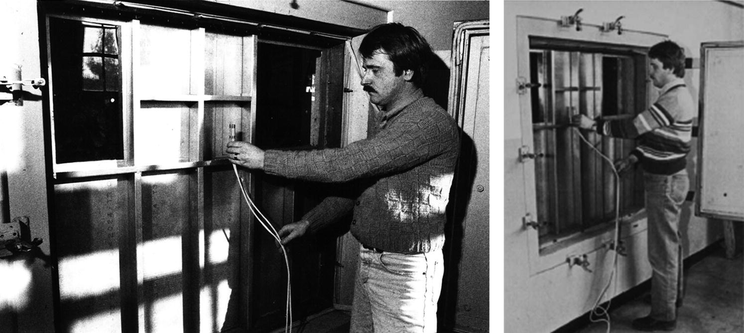
b) Round Robin Comparison of Transmission Loss
Figures 8.55 and 8.56 show the transmission loss results of a round robin test on two single‐leaf and double‐leaf constructions using the conventional two‐room method (Figure 12.30) and the sound intensity method (Figure 8.51).
c) Transmission Loss of Aircraft Structures
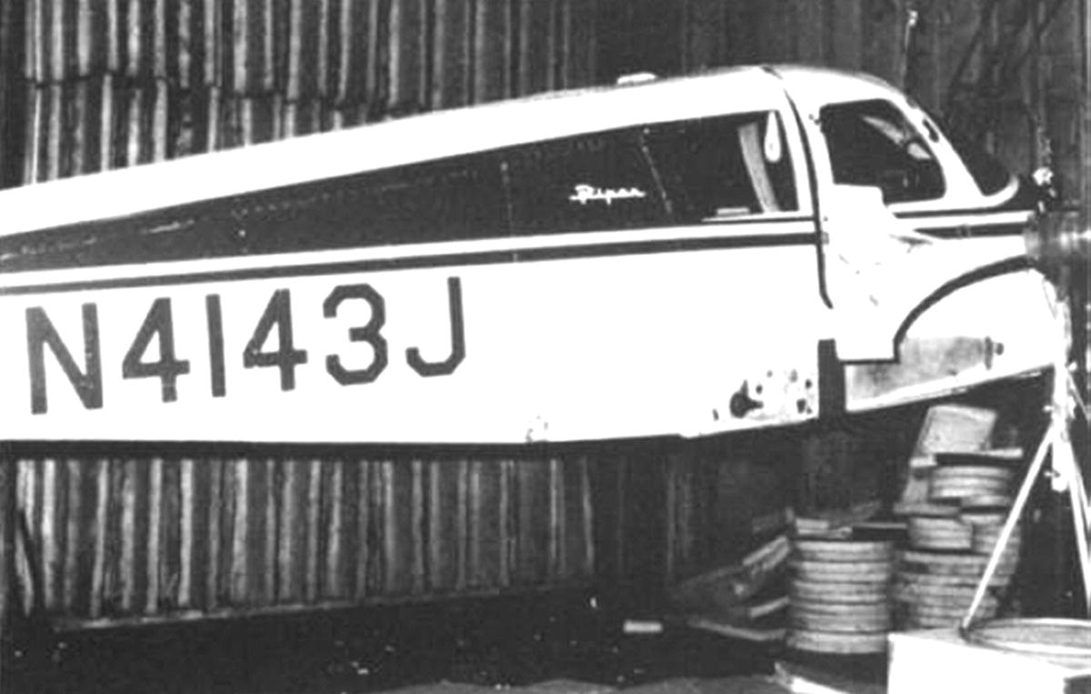
Sound intensity can also be used to study the transmission loss and radiation efficiency of engineering structures that are not flat and cannot be located in the window opening between two reverberation of transmission suite. Studies have been made on real aircraft structures such as a single engine Piper Cherokee [93, 99] (Figure 8.57) and a simulated half‐scale model of a light aircraft fuselage.
The sound transmission loss of different aircraft panels was measured in a semi‐anechoic chamber as well as in a reverberation chamber. These measurements represent normal incidence sound transmission loss and random incidence sound transmission loss, respectively.
In one set of measurements, the fuselage of the Piper Cherokee aircraft in Figure 8.57 was the subject of the tests. Four areas of the starboard fuselage sidewall were chosen for measurement studies; two single layer plexiglass windows and two aluminum panels with standard trim. One of the two plexiglass windows was part of the door unit, while the other was the passenger window behind the door. Similarly, one of the aluminum panels was located on the door under the window, while the other was located beneath the back passenger window.
For the measurement of normal incidence sound transmission loss, the fuselage was suspended from three points in the semi‐anechoic chamber with the bottom of the fuselage 1.37 m above the floor. The chamber itself is 12.5 m × 8.2 m × 5.5 m and has a concrete floor. To reduce reflections between the floor and the fuselage and to make the environment essentially anechoic, fiberglass sheets were placed on the floor beneath the fuselage. The acoustical excitation used was emitted from a pneumatic driver with a rectangular horn attached.
The instrumentation used to measure the sound transmission loss in the semi‐anechoic chamber is shown in Figure 8.58. To measure the sound intensity, half‐inch pairs of field‐incidence microphones (phase‐matched by Bruel and Kjaer on the basis of measurements in a pressure chamber), were arranged side‐by‐side with a spacing of 13.2 mm [99].
Figure 8.58 Instrumentation used for the measurement of sound transmission loss in the semi‐anechoic chamber: 1. Fuselage; 2. Phase‐matched microphones; 3. Microphone amplifiers; 4. Fast Fourier Transform Analyzer (FFT); 5 and 6. Horn and driver; 7. Amplifier; 8. Voltmeter; 9. Filter; 10. White noise generator; 11. Plywood‐Fiberglass divider [99].
The space‐averaged transmitted sound intensity for each panel and respective horn position was measured by sweeping the two‐microphone array over the interior of each panel of interest. Sweeping measurements were made as close as possible to each panel. A large amount of fiberglass was placed in the interior of the fuselage to make it reasonably anechoic for the sound intensity measurements. During the measurements inside the fuselage, the difference between the interior sound pressure level and the sound intensity level was monitored, and provided this difference did not exceed 12 dB, the interior transmitted sound intensity measurements were judged to be accurate. To prevent flanking of the panel under study, all panels having similar or lower sound transmission loss than the panel under study were covered with sheets of lead‐vinyl. The incident sound intensities for each panel and respective horn position were measured by removing the fuselage and sweeping the two‐microphone array over the same area as was previously occupied by the fuselage panel under investigation.
The random incidence sound transmission loss of the same four panels was measured with the fuselage suspended from three points in a reverberation chamber having dimensions 7.5 m × 6.2 m × 5.5 m. With the addition of the fuselage, the chamber was no longer truly reverberant. However, for the purpose of these tests, the sound field was considered to be sufficiently diffuse in the frequency range of interest, namely 100–1250 Hz [98].
The transmitted sound intensity was measured using a Bruel and Kjaer sound intensity probe (Type 3519) with a face‐to‐face microphone arrangement. To prevent sound entering the cabin via other parts of the fuselage, all parts except the starboard side containing the panels were covered with lead‐vinyl. The interior of the fuselage was made reasonably anechoic, and care was taken to prevent flanking of neighboring panels [98]. The sound intensity incident on the fuselage was assumed to be given by the diffuse field sound intensity:
(8.70)
where p2rms is the space‐average mean square sound pressure measured in the reverberation chamber using a half‐inch microphone rotating on a boom.
Figure 8.59 shows the comparison between the semi‐anechoic experimental results and mass law predictions in narrow 10 Hz bandwidths for the back window. The mass law predictions of the transmission loss seem to agree very well with those found experimentally. In the low frequency range, the transmission loss of a panel of this size is no longer mass‐controlled, as assumed in the mass law predictions, which may partly explain the observed discrepancy at low frequencies.
Figure 8.60 shows the one‐third octave band results for the sound transmission loss of the various panels under study. The two different aluminum panels with trim and the plexiglass windows seem to have nearly the same transmission loss up to about 400 Hz. It should be remembered, however, that at very low frequencies, (below 100 or 200 Hz) phase errors may lessen the accuracy of the results. Above the frequency of 400 Hz, the aluminum panels are seen to transmit considerably less sound power than the plexiglass windows.
d) Transmission Loss of Cylindrical Structures
Studies were made on aircraft models. In this study the fuselage structure was idealized as a cylindrical shell [95, 100]. An aluminium cylindrical shell of 0.76‐m diameter and 1.67‐m length was built. The boundary conditions of the cylindrical shell were intended to be fully clamped at the two ends of the shell and both ends were closed with massive end plates.
The dimensions of the cylinder were chosen to simulate a half‐scale model of a light aircraft fuselage. The incident intensity is obtained through the measurement of the diffuse field intensity in the transmission room or air space. Two cases have been studied. (i) The sound source was located inside the cylinder which was placed in an anechoic room. The interior sound field is assumed to be diffuse. (ii) The source was outside the cylinder which was placed in a reverberation room. In this second case, the interior of the cylinder was filled with fiberglass making it anechoic. In both the cases, the sound intensity transmitted from the exterior into the interior receiving space was measured using the two-microphone sound intensity method. Thus, in these two cases studied, the transmitting space was assumed to be reverberant and the receiving space anechoic.
To rate the sound transmission property of a cylindrical shell, the difference between the incident intensity level and the transmitted intensity level is desired. Figure 8.61 shows the set‐up with the sound source inside. In the second case the sound source was located outside in a reverberant room and the intensity was measured inside.
In the first case, the incident intensity was evaluated from Eq. (8.70) assuming the interior sound field to be diffuse. The average sound pressure inside the cylinder p2rms was measured by moving a microphone probe longitudinally and circumferentially inside the cylinder. The intensity transmitted through the cylinder from the interior to the exterior was measured outside using the sound intensity technique. The experimental results agree fairly well with the theoretical prediction in the higher frequency region. In the transmission suite method, it is assumed that the sound fields on the incident and transmitted sides of the structure are diffuse in nature. The assumption that the field inside the cylinder is diffuse in the present case cannot be satisfied in the low‐frequency range. This may explain the disagreement at low frequencies.
In the second case, the transmission loss was investigated by suspending the cylinder in a reverberation room. A very intense sound field was generated in the reverberation room. The central interior of the cylinder was filled with a large amount of 48 kg/m3 (3.0 lb./ft3) wedge‐shaped pieces of fiberglass to make the interior sound field as anechoic as possible. The two microphones were held so that the line joining their centers was in the radial direction and the microphone closer to the shell was 10 mm away from the surface. During the measurement the microphones were rotated circumferentially inside the cylindrical shell to obtain a spatially‐averaged sound intensity [95, 100].
The incident intensity in this case was measured by a single microphone mounted on a rotating boom in the reverberation room. Figure 8.62 shows narrow‐band plots of the transmission loss of the cylindrical shell as obtained in the two cases studied; (i) with the noise source in the cylinder and the transmitted intensity measured on the exterior surface of the cylinder when it was situated in an anechoic room and (ii) with the noise source outside the cylinder when it was situated in a reverberation room and the transmitted intensity measured on the interior surface of the cylinder which was filled with fiberglass and thus anechoic inside. Good agreement is found between the two plots in the high‐frequency region above 1500 Hz. Two dips in the transmission loss curve, one at the ring frequency (2100 Hz) and the other at the critical coincidence frequency (7500 Hz) are clearly observed.
The agreement between the transmission loss measurements when the noise source is either in the cylinder or exterior to it in the high‐frequency region also indicates that measurements can be done in either direction on a real aircraft fuselage providing that the incident field is diffuse and the receiving space is anechoic for both situations. For example, if only an anechoic chamber or a space out of doors without reflections is available, one can use an interior sound source and measure the transmitted intensity with the two‐ microphone method outside the fuselage, even though the real aircraft has noise sources outside the cabin.
The radiation efficiency indicates how efficiently sound is radiated from a structure to the acoustic field. It is defined as (see Chapter 3)
(8.71)![]()
where W is the sound power radiated from the structure, ρc is the characteristic impedance of the air, S is the surface area, and 〈v2〉 is the space‐averaged mean‐square velocity on the radiating surface.
The radiation efficiency of the cylinder can be determined by measuring the surface velocity of the vibrating structure and the sound power it radiates. The cylinder was excited by an external airborne noise source. The spatially averaged velocity was taken at 60 randomly distributed locations over the cylindrical shell. Figure 8.63 presents the one‐third octave band plot of the radiation efficiency measured over a frequency range of 50–10 000 Hz. Also shown in Figure 8.63 are the theoretical results of the radiation efficiency obtained from the wavenumber diagrams.
The agreement between the theoretical and experimental results seems to be fairly good – especially since the two peaks, one at the critical coincidence frequency and the other at the ring frequency, can be seen in the experimental radiation efficiency measurements.
Leave a Reply