Active and Reactive Sound Fields

As already discussed, in a one‐dimensional pure tone plane progressive wave the sound pressure and particle velocity are everywhere in phase for all values of time. The same situation exists far from idealized point sources of sound (monopoles, dipoles, quadrupoles, etc.) since the wave front curvature decreases and the surface becomes almost planar (flat) far from a source. However, close to the center of a source the situation is quite different and the sound pressure and particle velocity are almost completely 90° out of phase (in quadrature).

The near‐field behavior of simple discrete frequency sources is also sometimes studied by introducing the concepts of active and reactive sound fields. Four sound field quantities, potential energy density, kinetic energy density, active intensity and reactive intensity can be defined. These quantities were already described in the previous discussion of progressive plane wave propagation (Figure 8.5) and standing waves (Figure 8.6).

8.5.1 The Monopole Source

The active and reactive intensity can most easily be understood for a spherically spreading point source (or monopole) using trigonometrical functions. The sound pressure in outward traveling waves may be written (see Eq. (3.34)):

(8.25)

where Q is the source strength 4πa² U for a simple harmonic spherical source of radius a with normal velocity amplitude U. See Figure 8.8.

Here it is assumed that the source radius is small in wavelengths, a << λ, or ka << 1. The source strength Q has units of volume flow rate. The particle velocity u is everywhere radial and is given by

(8.26)

and thus, after integrating the results for ∂u/∂t, we obtain Eq. (8.27):

(8.27)

We notice that the first term represents the particle velocity, which is in phase with the sound pressure and is dominant far from the origin. The second term represents the particle velocity which is out‐of‐phase with the pressure and is dominant near to the source origin where r is small.

When kr << 1, the sound field is known as the near field; when kr >> 1, the sound field is known as the far field: when kr = 1, the in‐phase and out‐of‐phase particle velocity components are equal.

Upon multiplication of Eq. (8.25) with Eq. (8.27), we obtain the instantaneous sound intensity

(8.28a)

(8.28b)

We see that the fluctuating intensity at a distance r from the origin is comprised of two terms. The first term is seen to fluctuate at frequency 2ω but is always positive and represents energy flowing away from the source. The second term is also seen to fluctuate at frequency 2ω, but is alternatively positive and negative and represents energy flowing from and back toward the source. (See Figure 8.9 for kr = 1.)

When kr = 1, the real and imaginary intensity fluctuations are equal in magnitude. See Figure 8.9. When kr << 1, the imaginary term dominates; when kr >> 1, the real intensity term dominates.

EXAMPLE 8.1

A sphere of radius 5.5 cm pulsates with a surface velocity amplitude of 1.0 cm/s at the following frequencies: 50 Hz, 500 Hz, and 5000 Hz. Calculate (a) the volume velocity Q, (b) the distance to the near‐field/far‐field boundary at each frequency, (c) the magnitude of the real and imaginary intensity fluctuations at the boundary, and (d) the time‐average of the real and imaginary intensity components at the boundary.

SOLUTION

1. Q = 4πa² U = 4π(3.025 × 10⁻³) × (1 × 10⁻²) = 3.8 × 10⁻⁴ m³/s.
2. kr = 1, so r = 1/k = c/(2πf) = 344/(2πf). Then, r = 1.1 m at 50 Hz, r = 11 cm at 500 Hz, and r = 1.1 cm at 5000 Hz.
3. From Eq. (8.28), the magnitude of the real intensity fluctuation is (ρck² Q²/16π² r²) and the magnitude of the imaginary fluctuation is (ρckQ²/16π² r³). Therefore, at r = 1/k both magnitudes are equal to (ρck⁴ Q²/16π²). Thus, this magnitude is 2.6 × 10⁻⁷ watt/m² at 50 Hz, 0.0026 watt/m² at 500 Hz, and 26.1 watt/m² at 5000 Hz.
4. The imaginary intensity component given by the second term in Eq. (8.28) integrates to be zero over a period T = 2π/ω. The time‐average of the real intensity becomes: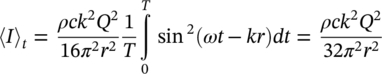. Now for kr = 1, 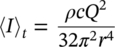. Thus〈I〉_t = 1.3 × 10⁻⁷ watt/m² at 50 Hz, 〈I〉_t = 0.0013 watt/m² at 500 Hz, and 〈I〉_t = 1.3 watt/m² at 5000 Hz.

EXAMPLE 8.2

Consider the same pulsating sphere of Example 8.1 and calculate its sound power at the frequencies 50 Hz, 500 Hz and 5000 Hz.

SOLUTION

The total sound power emitted by the source is found by integrating the time‐average real intensity over a sphere at some radius r (see Eq. (8.5)). Then,

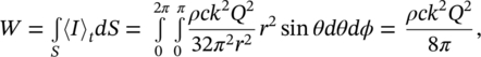 which is independent of radius as conservation of energy requires. Thus, the sound power of the pulsating sphere is W = 1.96 × 10⁻⁶ watt at 50 Hz, W = 1.96 × 10⁻⁴ watt at 500 Hz, and W = 1.96 × 10⁻² watt at 5000 Hz.

The fluctuating intensity is much more complicated for a dipole than a monopole, having more different regions and also an angular dependence, θ.

8.5.2 The Dipole Source

As discussed in Chapter 3, unlike the monopole, the sound pressure field produced by a dipole exhibits both near and far field behaviors (see Eq. (3.36)):

(8.29)

The first term represents sound pressure fluctuations in the near field and the second, in the far field. We notice again that the division between the two fields occurs when kr = 1.

The radial particle velocity can again be obtained from Eq. (8.26) and has three distinct regions. The radial sound intensity fluctuations are obtained by multiplying the pressure by the velocity (see Eq. (3.40)).

8.5.3 General Case

In general, the active intensity I is defined to be the product of the sound pressure and the in‐phase radial particle velocity and the reactive intensity J is defined to be the product of the sound pressure and the out‐of‐phase component of the radial particle velocity. Using complex notation, the real (active) and imaginary (reactive) components of the sound intensity are

(8.30a)

(8.30b)

The reactive intensity J is thus a vector quantity with a direction (like the active intensity) pointing away from the source in the radial r‐direction. However, by definition it is seen that it has a long time average of zero at any point in the sound field. The reactive intensity has been misinterpreted by some making it a somewhat controversial subject. This may be because when it is plotted, it is usually shown as an arrow (of length representing its magnitude) and direction away from the source. Thus, some have assumed it represents a real flow of energy, instead of a fluctuating flow, from and to a point in the sound field. Perhaps a two‐headed arrow representation could be better with the arrow heads at each end pointing away from and also back toward the point in the field.

It has been shown mathematically that the real active intensity can be written as [28, 29]

(8.33)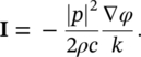

The active intensity has a direction orthogonal (perpendicular) to surfaces of constant phase (wave fronts). It is seen immediately that it is very important to avoid phase errors in the measurement of sound intensity.

The reactive intensity can be written as [28, 30]

(8.32)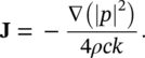

The reactive intensity is thus seen to be proportional to the gradient of the mean square pressure. It is orthogonal to surfaces of equal sound pressure. Because the active and reactive intensities are given mathematically by the real and imaginary parts of the product of the sound pressure and the complex conjugate of the particle velocity, the term complex intensity has been defined and used by some:

(8.33)

With the advent of the cross‐spectral method of measurement of sound intensity in the late 1970s [31, 32], interest grew in theoretical modeling of sound fields. Pascal published an early analytical study in 1981 concerning active and reactive sound intensity and coined the term complex intensity [29], Tichy and his colleagues extended this analytical study in 1984 and 1985 [33–36].

Some have found these theoretical studies not to have been very helpful or even have been confusing for practitioners who use sound intensity in engineering problems for sound power measurement and sound source identification of machinery. There are two main reasons: (i) these studies have mostly concerned idealized single‐frequency sound sources (the particle velocity can only be separated into components in phase and out of phase with the sound pressure for discrete frequency sources), and (ii) the plots of reactive sound intensity are represented by arrows of different lengths (normally pointing away from sources): the lengths correspond to the fluctuation magnitude at these locations. Jacobsen has pointed out that the direction of the reactive intensity arrows is related to the spatial derivative of the square of sound pressure only and could equally well be shown in the reverse direction. As already stated, it has been suggested that this confusion would be overcome by replacing the single direction arrows with double headed arrows showing both directions of the pulsating energy flow.

In 1984, Elko and Tichy suggested that the reactive intensity, which is known to be high near sources, could be useful in noise source location [34]. However, Crocker pointed out at that time that in the ideal case of a pure tone standing wave in a tube (see Figure 8.6) the reactive intensity is high, although no source is present [25, 37]. The same situation exists for the ideal case of standing waves in a room with hard walls in which no source is present. Indeed Pascal has emphasized that when sources are present, “(reactive intensity) cannot be used directly to locate sound sources; (this is) because interference situations obliterate the assumption that the decrease of (the) reactive intensity vector indicates source positions” [38]. Pascal gives an example of the interference of a plane wave and a near‐field wave [38]. He goes on to say “A general answer to the source identification problem will only be given by a detailed study of active intensity potentials (scalar and vector).”

Although separating the particle velocity in a sound field into components that are in phase and out‐of‐phase with the sound pressure can strictly be done only for discrete frequency sounds, Jacobsen used this approach with one‐third octave band random noise signals [28]. The approach required the use of the Hilbert Transform as formulated by Heyser [40] Jacobsen [28] made measurements in the sound field, near a loudspeaker, a vibrating box and in a reverberation room. The measurements were made in the near field at varying distances from the source: near field, 30 and 50 cm in one‐third octave bands centered at 240 Hz, 500 Hz, and 1 kHz. The results are said to represent the running short‐time average of the active and reactive components of the complex instantaneous intensity [28]. The time windows used vary from 31.25 to 125 ms. The results obtained are not easy to interpret. By definition, the instantaneous reactive intensity should average to zero if a sufficiently long time window is taken. Since this was not the case, it suggests that sufficiently long averaging times need to be used in practice to obtain a reliable and repeatable value of the mean sound intensity. Fahy also reached this conclusion in evaluating Jacobsen’s results [24]. Kutruff and Schmitz commented in 1994 that “the measurement of sound intensity (has) so far not found the practical application it deserves” [41]. They commented that one possible reason is the conceptual difficulty inherent in (interpreting) the intensity (a vector). They also went on to say that “the frequently made distinction between ‘active’ and ‘reactive’ intensity may have added to the confusion about intensity” [41].