VELOCITY DIAGRAMS FOR IMPULSE STEAM TURBINE

Let u = circumferential or tangential linear velocity of blades

   v_a1 = absolute velocity of steam at inlet of moving blade

   v_a2 = absolute velocity of steam at outlet of moving blade

   v_w1 = velocity of whirl at the entry of moving blade

      = v_a1 cos α₁

   v_w2 = velocity of whirl at the exit of moving blade

       = v_a2 cos α₂

   v_f 1 = velocity of flow at inlet of moving blade

       = v_a1 sin α₁

   v_f 2 = velocity of flow at outlet of moving blade

       = v_a2 sin α₂

   v_r1 = relative velocity of steam at entrance to moving blade

   v_r2 = relative velocity of steam at exit of moving blade

   ṁ = mass rate of flow of steam, kg/s.

   D = diameter of blade drum.

   h = height of blade.

   α₁ = angle which the absolute velocity of steam at inlet makes with the plane of moving blades, or nozzle angle or outlet angle of fixed blades.

   α₂ = angle which the absolute velocity at outlet makes with the plane of moving blades or inlet angle of fixed blade.

   β₁ = inlet angle of moving blade.

   β₂ = exit angle of moving blade.

The jet of steam impinges on the moving blades at angle α₁ to the tangent of wheel with a velocity v_a1. This velocity v_a1 has the following components.

1. Tangential or whirl component v_w1 and since it is in the same direction as the motion of blades, it is the actual component which does work on the blade.
2. Axial or flow component v_f 1 and since it is perpendicular to the direction of motion of blade, it does no work. However, this component is responsible for the flow of steam through the turbine. This component also causes axial thrust on the rotor.

The velocity diagrams at inlet and outlet of a moving blade are shown in Fig. 7.6(a). Figure 7.6(b) shows the combined velocity diagrams.

Figure 7.6 Velocity diagrams for impulse turbine: (a) Velocity diagrams at inlet and exit, (b) Combined velocity diagrams

For blades with a smooth surface, it can be assumed that friction loss is very less or zero. However, there is always a certain loss of velocity during the flow of steam over the blade and this loss is taken into account by introducing a factor called blade velocity coefficient, K. It is given by

 

Blade velocity coefficient, K = v_r2/v_r1, where v_r2 < v_r1.

Note that K accounts for the loss in relative velocity due to friction of blades.

1. Power Developed by the Turbine:Work done per kg of steam,w = Force in the direction of blade motion × Distance travelled in the direction of force    = Rate of change of momentum × Distance travelled    = [v_w1 − (− v_w2)] × u    = (v_w1 + v_w2) uPower developed by the turbine for a mass rate of flow of ṁ kg/s of steam,
2. Diagram or Blade Efficiency, η_d or η_b:For a single blade stage, 
3. Gross or Stage Efficiency, η_s:  Stage efficiency takes into account the losses in the nozzle. 
4. Axial Thrust: The axial thrust on the wheel is generated due to the difference between the velocity of flow at inlet and outlet.Axial thrust, F_a = Mass rate of flow of steam × Change in axial velocity
5. Energy converted into heat due to blade friction:= Loss of kinetic energy during flow of steam over the blades
6. 

1 Condition for Maximum Blade Efficiency

Blade efficiency, 

From velocity diagrams given in Fig. 7.6(b), we have

where 

Now BE = AE − AB = v_a1 cos α₁ − u

Let speed ratio, 

For η_b to be maximum, 

∴ cos α₁ − 2ρ = 0

For symmetrical blades, β₁ = β_2, so that C = 1 and with no friction over the blades, K = 1

2 Maximum Work Done

Now, w = (v_w1 + v_w2)u

Equations (7.11) and (7.12) represent parabola. The blade efficiency has been plotted against speed ratio in Fig. 7.7, without losses and with losses for α₁ = 20°, β₁ = β₂ and K = 0.85.

Figure 7.7 Blade efficiency v’s speed ratio

3 Velocity Diagrams for Velocity Compounded Impulse Turbine

The velocity diagrams for the first and second stage moving blades of a velocity-compounded impulse turbine are shown in Fig. 7.8(a) and Fig 7.8(b), respectively. Consider that the final absolute velocity of steam leaving the second row is axial. The velocity u of the blades for both the rows is the same as they are mounted on the same shaft and are of equal height.

Work done in the first row of moving blades,

 

w₁ = u(v_w1 + v_w2) = u(v_r1 cos β₁ + v_r2 cos β₂)

If there is no friction loss, v_r1 = v_r2 and for symmetrical blades, β₁ = β₂.

∴ w₁ = 2u v_r1 cos β₁ = 2u(v_r1 cos α₁ − u)

Now, v_a3 = v_a2

Work done in the second row of moving blades,

 

w₂ = u v_w3 as v_w2 = 0 and a₄ = 90°.

= u (v_r3 cos β₃ + v_r4 cos β₄)

Figure 7.8 Velocity diagrams for velocity compounded impulse turbine: (a) First stage, (b) Second stage

For no friction, v_r3 = v_r4, and for symmetrical blades, β₃ = β₄.

∴ w₂ = 2uv_r3 cos β₃ = 2u (v_a3 cos α₃ − u)

For α₃ = α₂

 

v_a3 cos α₃ = v_a2 cos α₂

= v_r2 cos β₂ − u = v_r1 cos β₁ − u

= (v_a1 cos α₁ − u) − u = v_a1 cos α₁ − 2u

∴ w₂ = 2u [(v_a1 cos α₁ − 2u) − u] = 2u (v_a1 cos α₁ − 3u)

Total work done, w_t = w₁ + w₂

 

= 2u (v_a1 cos α₁ − u) + 2u (v_a1 cos α₁ − 3u)

= 2u (2v_a1 cos α₁ − 4u)

= 4u (v_a1 cos α₁ − 2u)

Blade efficiency, η_b =

For η_b to be maximum,

 

cos α₁ − 4ρ = 0

 

For 

where n = number of rotating blade rows in series.

4 Effect of Blade Friction on Velocity Diagrams

In an impulse turbine, the relative velocity at the outlet will be the same as the relative velocity at the inlet, if friction is neglected. In practice, there is a frictional resistance to the flow of steam jet over the blade, the effect of which is to cause a slowing down of the relative velocity. Usually, there is a loss of 10−15% in the relative velocity due to friction. Owing to frictional resistance of the blades, it will be found that v_r2 = Kv_r1, where K is a coefficient, which takes the blade loss due to friction into account. The velocity diagrams considering blade friction are shown in Fig. 7.9. Here, the inlet diagram is first drawn and the line BC, of an unknown length, is drawn at the correct angle β₂. Mark off on line BD = v_r1, the friction loss of relative velocity DD′, then BD′ = Kv_r1. With B as centre, draw an arc of radius BD′ to cut BC at C. Then BC = v_r2 = Kv_r1.

By joining A and C, the line AC representing v_a2 is obtained. This completes the outlet velocity diagram.

Figure 7.9 Velocity diagrams for impulse turbine considering blade friction

5 Impulse Turbine with Several Blade Rings

The stage of an impulse turbine, which is compounded for velocity, consists of alternate rings of nozzles, and moving and fixed blades. As the blade velocity u is constant for all the moving blade rings of the stage, the velocity diagrams for all the blade rings can be superimposed on the same base, represented by u. Figure 7.10 shows the velocity diagram for a stage consisting of two moving and one fixed blade rings. Let us assume that the following data is known:

1. Blade velocity, u.
2. Nozzle angle, α₁.
3. The moving blade angles, β₁ and β₂, which are assumed to be same for both blade rings.
4. The velocity of steam v_a1 discharged from nozzle.
5. Blade friction loss, 10%, i.e., K = 0.9.

The following steps may be followed for drawing the velocity diagrams:

1. Draw AB = u to any convenient scale. Draw AD inclined at angle α₁ to AB so that AD = v_a1 to the same scale. Join BD. Then BD = v_r1 for the first moving blade ring.
2. Mark off DD′ = 0.1 × BD so that v_r2 = 0.9 v_r1 = BD′. With B as centre, draw an arc of radius BD′ to cut BC at C where the line BC is drawn at angle of β₂ to BA. Join AC. Then AC = v_a2 for the first moving blade ring.
3. The steam now flows over the fixed blade ring and will lose 10% of its velocity during the passage. Hence, mark off CC′ = 0.1 × AC. With A as centre, draw on arc of radius AC′ to cut BD at G. Then AG = v_a3 representing the steam velocity when entering the second moving blade ring. The velocity diagram for the second blade ring is triangle AGB. BG = v_r3, the relative velocity. 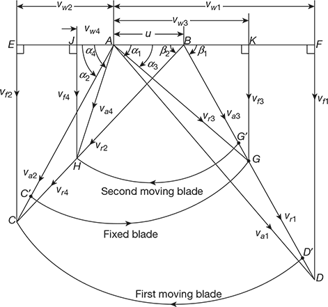Figure 7.10 Velocity diagrams for impulse turbine considering friction with several blade rings
4. The steam now flows over the second moving blade and loses one-tenth of its relative velocity due to friction., Hence, mark off GG′ = 0.1 × BG so that BG′ = 0.9 BG. With B as centre and radius BG′, draw an arc to cut BC at H, then AH = v_a4 and BH = v_r4.α₂ = angle of discharge from first moving bladeα₄ = angle of discharge from second moving bladeα₃ = outlet angle of fixed blade.Work done per kg of steam for first moving blade ring, w₁ = (v_w1 + v_w2)uWork done per kg of steam for second moving blade ring. w₂ = (v_w3 + v_w4)uTotal Work done, w_t = w₁ + w₂ = [(v_w1 + v_w2) + (v_w3 + v_w4)]uPower developed per stage = Blade efficiency, η_b = Stage efficiency, η_s = Total axial thrust =