Sound and Vibration Transmission and Structural Response Using Statistical Energy Analysis (SEA)

12.4.1 Introduction

Statistical Energy Analysis is often abbreviated to SEA. SEA was first used in the early 1960s to predict the vibration response of aerospace structures to acoustical environments and to determine the transmission of acoustical and vibrational energy in such structures [21–26]. Ungar, Eichler, Lyon, Maidanik, Smith, Scharton and Manning were some of the main contributors. In 1969, 1970, and 1971, Crocker, Price, and Battacharya published a theoretical approach to predict the sound transmission through finite single and double panels and later panels connected by tie beams [27–30]. The SEA approach has the advantage that (i) sound absorption in the double‐panel air gap cavity and (ii) double‐panel bridges can be accounted for, theoretically [30].

SEA relies heavily on several results, which have been known in acoustics for many years, such as the modal density and the acoustic energy density of systems. However, one additional result is the assumption that the energy flow between two coupled systems is proportional to the modal energy difference between the two systems [21–26]. In SEA, although the panels and air spaces are assumed to be finite, and modes are assumed to exist in the structures, space–time and frequency averages are made early in the analysis. This enables much simpler solutions to be found than in classical modal analysis theory, which is an alternative approach. For further details about SEA theory, the reader is directed to the books and book chapters by Lyon [21] and De Jong [31], Norton [32], Fahy and Walker [33], Nilsson and Liu [34], Keane and Price [35], Manik [36], and Hambric and Le Bot [37, 38].

SEA has now been applied to a variety of acoustics and vibration problems. More details of SEA theory and its applications to the solution of sound transmission loss problems are given by Crocker and colleagues in journal papers [27–30]. Thus, only a very brief account of the theory – and mainly its applications to sound transmission problems – will be considered in the present Section 12.4.2 of this chapter.

12.4.2 SEA Fundamentals and Assumptions

In order to solve complicated sound/structure response problems, it is necessary to make simplifying assumptions. In SEA these normally involve making averages over time, space and frequency. It is beyond the scope of the discussions in this chapter to go into great depth. Several papers, books and book chapters provide the necessary background [21–26, 31–46]. The NASA CR‐160 report by Smith and Lyon is particularly useful [23]. SEA works best at high frequency when there are many modes (in structures and air spaces) resonant in the frequency band under consideration.

When a structural/cavity system is excited by broadband noise, modes of vibration are excited in both the structure and the coupled air cavities. At high frequency, it is found that the shape of the structural panels and of the air cavities is not very important. In most cases the areas of the structural elements and volumes of the cavities are more important than their shapes. Some elementary discussion about the modal behavior of structural panels and air cavities is also included in Sections 3.16 and 3.17 of this book.

• a) Vibration of a Simple SystemIt is assumed that the vibration of extended flat plate structures is almost entirely in bending and it can be modeled as a set of simple resonators. In more complicated built‐up structures, however, it is common to include in‐plane vibration in SEA models. In steady‐state forced vibration, a resonator possesses both kinetic energy T = ½Mv²(t) and potential energy U = ½Kx²(t) and in steady‐state vibration 〈T〉_t = 〈U〉_t, where 〈 〉_t represents a long‐time average and is often shortened to 〈 〉 (see Eq. (1.7)). In SEA another energy term is of most importance, the dissipated power W_diss = R〈v²〉_t. Here R is the resistance, and Rv(t) is the resistive force f_R(t), so that W_diss = f_R v(t) = 2D, where D is the Rayleigh dissipation function. For steady state, 〈W_diss〉 = R_diss 〈v²(t)〉.
• b) Energy Loss FactorWe assume small viscous damping for the resonators. Thus, we can write: 〈W_diss〉 = R〈v²〉 = ηω_n M〈v²〉 = ηω_n〈E〉 = β〈E〉, where η is the loss factor and β = the energy loss factor. For transient vibration we can write: 〈E〉 = E₀ e^−ωt, where E₀ is the energy at time t = 0. Thus η = 〈W_diss〉(ω_n〈E〉), where the loss factor η represents the energy dissipated in one cycle of 2π/ω_n seconds. In acoustics, we define the reverberation time T_R to be the time in which the energy level in the sound field decays by 60 dB. Likewise in vibration, we write T_R = 2.2/(ω_n) seconds. Here f_n = ω_n/2π is the natural frequency of the resonator, Hz.
• c) Modal Densities of Beams, Plates and RoomsThe modal densities of coupled structures and air spaces are of considerable importance in SEA. For convenience, we normally assume simple supports for the structures and hard walls for the air spaces for mathematical simplicity. At high frequency, the structural and air spatial boundary conditions are found to be of only secondary importance. The modal density can be given in terms of angular frequency ω, rad/s or frequency f, Hz. The modal density represents the number of modes with natural frequencies per radian/second or per hertz, and of course normally depends on frequency.
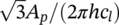
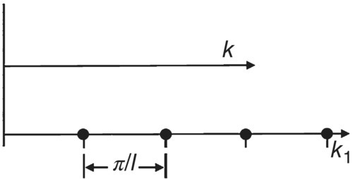
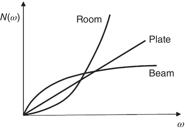
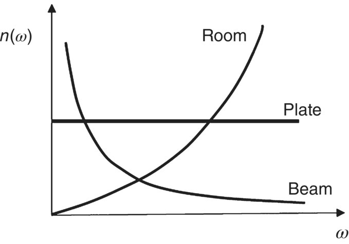
  1. For a beam:The natural frequencies for a simply‐supported beam of length l are given by ω_m = κc_L k²_m, where k²_m = (mπ/l)².The number of modes N(k) below wavenumber k is from Figure 12.12, N(k) = k/(π/l), and from the above equations: N(ω) = (ω^1/2 l)/[π(κc_L)^1/2].N(ω) is the total number of modes below frequency ω. The number N(ω) increases with ω^1/2. The modal density n(ω) may be obtained by differentiating: n(ω) = l/[2π(ωκc_L)^1/2]. The modal density of a beam is proportional to its length and decreases with frequency according to ω^−1/2.For a thin plate:The natural frequencies for a simply‐supported rectangular plate, of length and width l₁ and l₂, are given by ω_m = κc_L k_m², where k_mn² = k_m² + k_n² = (mπ/l₁)² + (nπ/l₂)².The number of modes below wavenumber k is from Figure 12.13, N(k) = (π k²/4)/(π²/ (l₁ l₂)) = k² A_p/(4π), thus N(ω) = (ωA_p)/(4πκc_L), which increases with ω. The modal density n(ω) may be obtained by differentiation. 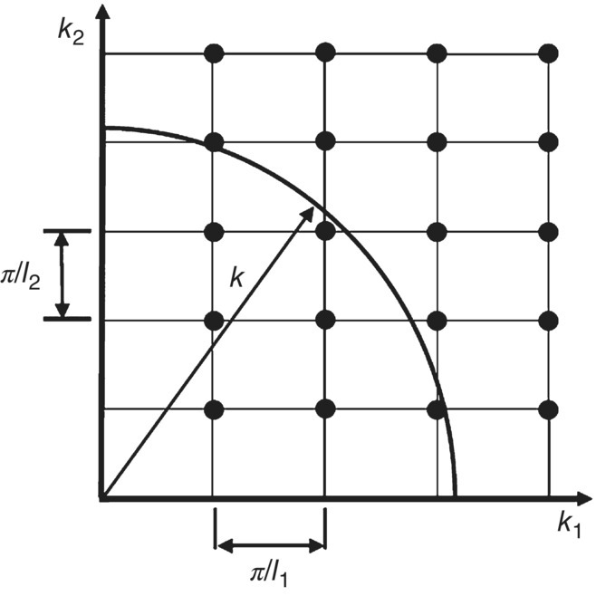Thus, the modal density n(ω) = A_p/(4πκc_L) = , which is seen to be a constant and only depends on the plate area A_p. It should be noted, however, that the modal density of thick and sandwich plates depends on the effective wave speed and is more complicated to compute [47].For a room:The natural frequencies in a rectangular hard‐walled room are ω_m = ck, where k = [(mπ/l₁)² + (nπ/l₂)² + (lπ/l₃)²]^1/2, c is the speed of sound in air and l₁, l₂, and l₃ are the room length, width and height.The number of modes N(k) below wavenumber k (at high frequency ignoring longitudinal and lateral modes) can be obtained from Figure 12.14, N(k) = (πk³/6)/(π²/(l₁ l₂ l₃)) = k² V/(6π²) and thus, N(ω) = ω³ V/(6π³ c³) which increases as ω³.Thus, by differentiation the modal density is n(ω) = ω² V/(2π² c³). The modal density of a room is proportional to its volume and the square of frequency. The mode count N(ω) and modal density n(ω) results above are plotted in Figures 12.15 and 12.16.
  In acoustics the modal density n(ω) is important for several reasons. In structural response and radiation, if n(ω) is high we can use statistical approaches. If n(ω) is very low, (only a few modes in the frequency range of interest) we must use the classical approach and work out the response (or radiation) for each mode separately and then sum the modal contributions. In a reverberation room, if there are only a few modes resonant (in say a 1/3 octave band) there will be large fluctuations in panel or air cavity response with the position. This limits the use of SEA to high frequencies.
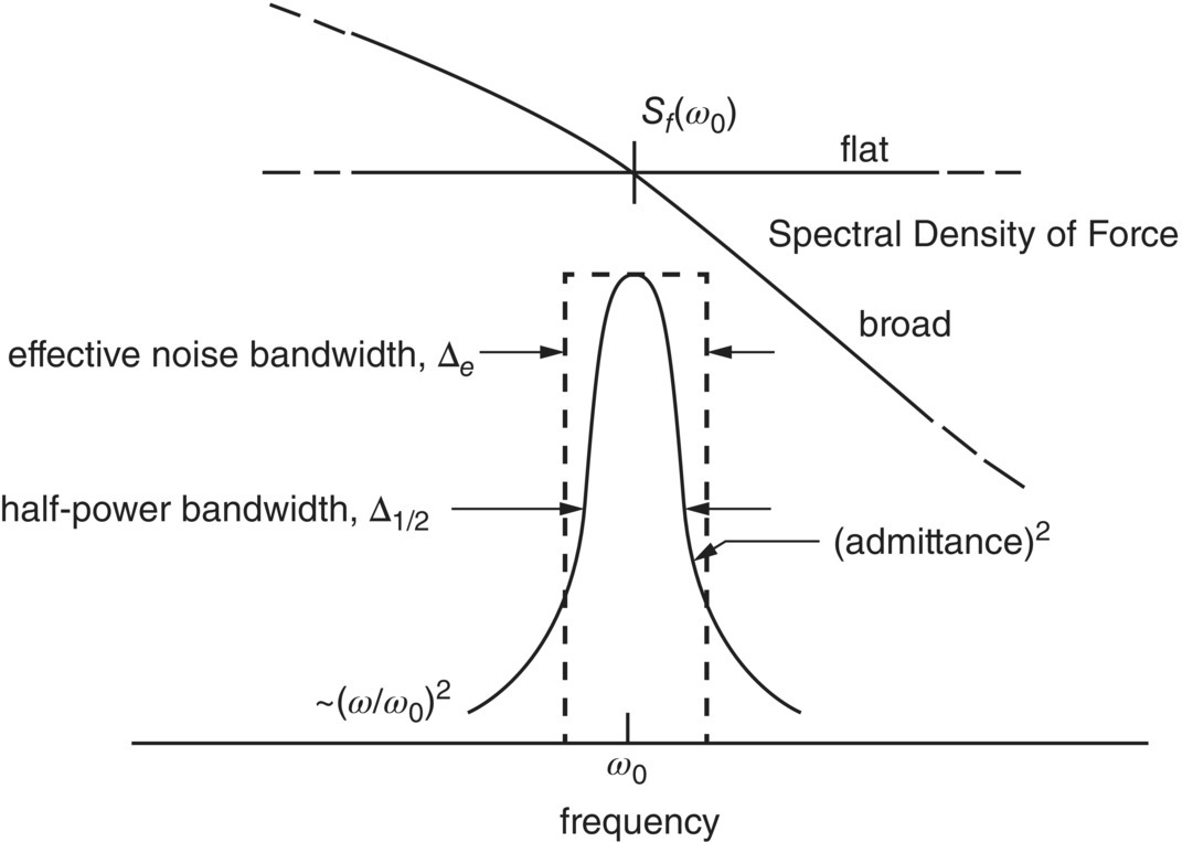
• d) Half Power Points and BandwidthAssuming a resonator is excited by a pure tone, we can relate the magnitude of the velocity response V to the magnitude of the force F by its impedance Z = F/V. Both the force F and velocity V can, in general, be complex and contain both magnitude and phase information. Often, we desire the inverse of the impedance 1/Z = Y, the so‐called admittance. At resonance, the admittance becomes real and is called the conductance G. The mechanical engineer’s critical damping ratio δ (see Eq. (2.16)) is related to the loss factor by δ = η/2. The resonator bandwidth Δ_1/2 is given by the difference in the half power points Δ_1/2 (ω) = ηω_n = 2δω_n.If the resonator is excited by a stationary broadband noise source of spectral density S_f (ω) (see Eq. (1.12)), then a new “effective bandwidth” Δ_e can be defined as Δ_e = π/2ω_n η = π/2R/M = π/2Δ_1/2. See Figure 12.17. Also see Ref. [23].
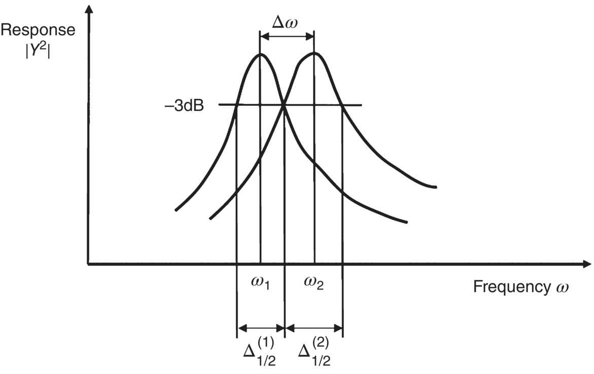
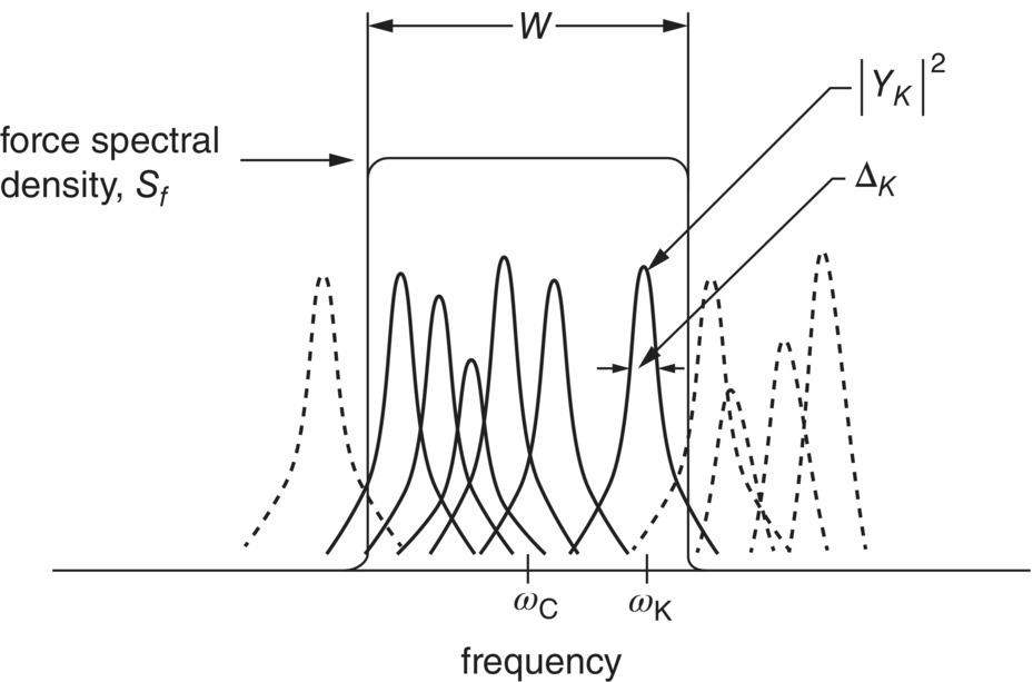
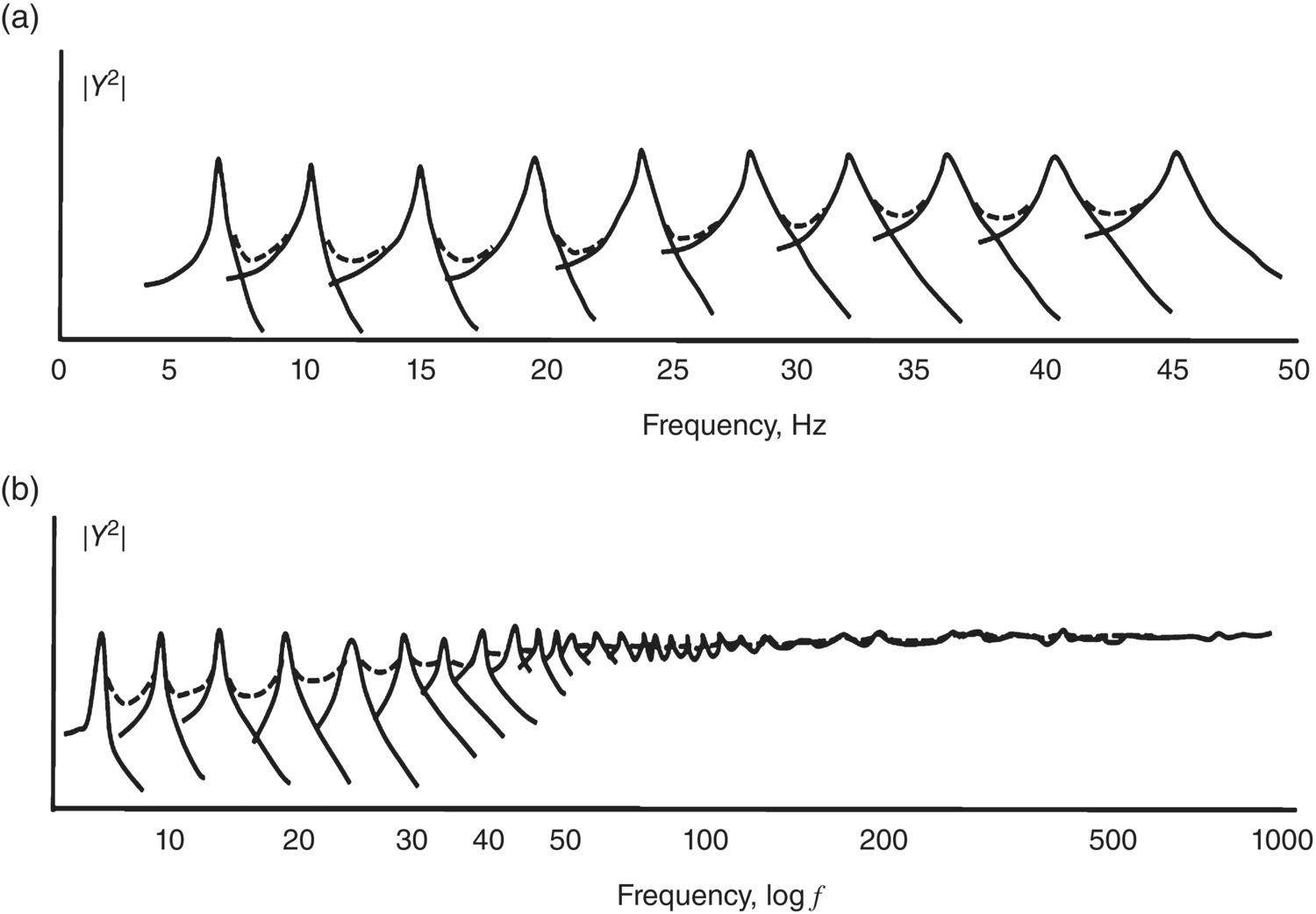
• e) Modal OverlapWe can see that for a constant value of η, which is assumed to be independent of frequency, both the half‐power points bandwidth Δ_1/2 and the effective bandwidth Δ_e of an average mode increase with frequency ω. A frequency is reached where the frequency separation of modes Δω_n on a two‐dimensional structure becomes equal to or less than the half‐power bandwidth Δ_1/2 = ηω_n of an average mode. Figure 12.18 shows two closely‐spaced modes subjected to pure tone excitation. Here we see that the half power bandwidth ω_1/2 of mode number ω₁ does not exceed the modal frequency separation, Δω. However, it has become equal to that for mode number ω₂ and by the next mode ω₃, it is expected that the half power bandwidth of the mode of center frequency ω₃ will exceed the frequency separation Δω.In cases when structures are excited by broadband noise, it is more realistic, however, to use broadband noise excitation rather than pure tone excitation in defining the modal overlap frequency f_over. In this case, the modal overlap frequency occurs when the average modal frequency separation Δω_n equals the effective noise bandwidth Δ_e of a typical resonance. That is when Δω_n = π/2ηω_n. See Figure 12.18 in which the magnitude of the admittance squared |Y|² is plotted against frequency ω. Both the half power bandwidth Δ_1/2 and the effective noise bandwidth Δ_e are shown for force excitation of spectral density S_f(ω) in Figure 12.18.It is often stated that SEA works well only if the modal overlap factor is greater than unity. However, this statement is not correct if SEA is viewed in Lyon’s original sense as an ensemble theory (R.S. Langley, personal communications, June 21 and 22, 2019). That is the method considers an ensemble of random systems and the predicted energies must be interpreted as ensemble average values. The energy in any one member of the ensemble may differ from the SEA prediction, because the energy has a variance across the ensemble. If the modal overlap is high, then the ensemble variance is low, and every member of the ensemble will have approximately the same energy. But this does not mean that SEA fails when the modal overlap is low – the ensemble average energy can be predicted accurately (R.S. Langley, ibid).The mean energy is predicted extremely well for very low values of modal overlap (typically as small as 0.5), and the variance can still be predicted well. The variance theory is based on Ref. [49]. So it does not follow that SEA only works for high values of modal overlap. The variance theory can also be applied to coupled FE/SEA models [49] (R.S. Langley, ibid).Statistical overlap is also important. That is the degree of randomness in the structure for the ensemble theory of SEA to hold requires that there must be sufficient randomness in the system. The statistical overlap is a measure of the rms change in a natural frequency across the ensemble compared to the mean natural frequency spacing (i.e. the “bandwidth” used in the definition of modal overlap is replaced by the rms change in the natural frequency). SEA tends to work when the statistical overlap is greater than unity [49] (R.S. Langley, ibid.). This sets a lower frequency limit on the method, but the modal overlap may be extremely small at this limit [49] (R.S. Langley, ibid.).Figure 12.19 shows the admittance squared response, |Y|² of a set of resonators excited in a frequency band W by a force of constant spectral density S_f. As the center frequency ω_c increases, the effective bandwidth of mode number k, Δ_k = ½πη_k ω_k also increases. In the case of a flat panel, the average mode separation, Δf_mode, is independent of frequency. The net result is that, if the panel loss factor η remains constant with frequency, the resonance peaks are distinct and separate at low frequency, but become less and less distinct as the frequency increases above the modal overlap frequency f_over. See Example 12.8, part (d). This effect is illustrated in Figure 12.20, where the simplifying assumption is made that the modes have the same frequency separation and all respond with equal energy to the force excitation.
• f) Radiation Resistance of a Panel

There are several ways to evaluate the response of a simply‐supported panel to noise and the power radiated by the panel when it is excited by noise. We shall assume that either (i) all modes in the frequency band considered have the same mean square velocity (sometimes called equipartition of energy), or (ii) all modes in the band have the same radiation resistance. For modes below the critical frequency, we shall make the first assumption, and for modes above the critical frequency f_c we shall make the second assumption.

The study of finite simply‐supported panels has suggested that the major source of radiation from the panel below the critical frequency arises from the interactions of bending waves with edge discontinuities. In particular, those modes of vibration which result in a trace flexural wavelength along the edges, which is greater than the acoustic wavelength, are responsible for most of the radiation from these edges. When the trace flexural wavelength in both directions is greater than the acoustic wavelength, then the corners of the panel alone radiate. Normally these “corner modes,” however, radiate much less than the so‐called “edge modes” and their contributions can be neglected.

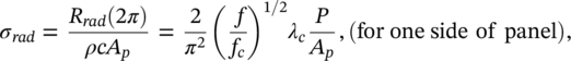
In the analysis presented here, it is assumed at all stages that the panel dimensions are greater than the acoustic wavelength. This simplifies matters in that the interactions between canceled volume velocity elements at the edges and corners of the panel can be treated independently. If the panel dimensions are smaller than the acoustic wavelength, then these simple radiators interact. This case has been considered by Maidanik [39] who, by treating the problem in more depth than is possible here, has derived the equations given in Ref. [39] and in corrected form in Refs. 27, 28. 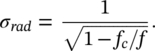The following simple formulas for radiation to half space for the acoustically slow (A.S.) radiation of a panel below and the acoustically fast (A.F.) radiation above the critical frequency f_c are  = (f/f_c)^1/2 (ρcλ_c P)/π², when f < f_c/2, and where P is the perimeter of the whole panel. For radiation above f_c,  = ρcA_p(1−f_c/f)^−1/2. Note that Smith and Lyon give a result for the A.S. radiation in Ref. [23] (Eq. VI.4.2) which is eight times larger and is assumed to be in error [23].

It is of interest to note that the average radiation resistance below the critical frequency is directly proportional to the perimeter P and not to the area A_p of the panel. These results are, of course, only strictly valid for simply‐supported panels. It has been shown by Nikiforov that for f < f_c the radiation resistance of a panel with clamped boundaries will give rise to far field mean‐square sound pressures twice those for the simply‐supported panel.

EXAMPLE 12.8

The walls between the engine room and a storeroom on a passenger ship are made of 1/16 in (1.6 mm) thick steel. One partition panel wall under consideration measures 3 ft × 4 ft (0.91 m × 1.22 m). Calculate:

1. The approximate critical coincidence frequency;
2. The modal density of the panel;
3. The number of modes in one‐third octave bands centered at 10, 100, 1000 and 10000 Hz.
4. The modal bandwidth; assuming the panel damping is 0.5% critical and independent of frequency
5. The lowest natural (resonance) frequency of the panel, and
6. The frequency range in which the panel is acoustically large l_min > λ.

SOLUTION

The solutions are worked in English and SI units. Both systems give the same results. The panel is assumed to have simply supported edges. This is a good engineering assumption to make at high frequency since the boundary conditions have little effect on mode shapes and the panel natural frequencies. This is because most of the vibration takes place away from the boundaries. The working assumes that space‐averaging is made over the panel and in the air space contiguous to it.

1. The critical coincidence frequency, , where c = speed of sound = 1116 ft/s = 343 m/s and κ is the panel radius of gyration.For aluminum and steel, the longitudinal wave speed c_L =17000 ft/s = 5280 m/s.Substituting for c, and  for steel and aluminum, where h = panel thickness in inches, gives
2. The modal density, n_p for a simply‐supported panel is given byThus n_p(f) = 2π × 0.037 modes/Hz. (Remember 1 cycle = 2π rad and 1 Hz = 1 cycle/s = 2π rad/s). Thus, modal density n_p(f) = 0.235 modes/Hz.
3. The frequency bands for one‐third octaves are given by ∆f = 23% f_cent, where f_cent is the center frequency for the band (see Chapter 1).Thus, the number of modes n in a band is given by n = n_p(f) × 0.23 f_cent
   1. f_cent = 10 Hz, n = 0.235 × 10 × 0.23 = 0.54 modes
   2. f_cent = 100 Hz, n = 0.235 × 100 × 0.23 = 5.4 modes
   3. f_cent = 1000 Hz, n = 0.235 × 1000 × 0.23 = 54 modes
   4. f_cent = 10000 Hz, n = 0.235 × 10000 × 0.23 = 540 modes
4. The Effective Modal Bandwidth, b(f) = (π/2)η_int(2πf). But if the critical damping ratio δ = 0.005, then the internal energy loss factor, η_int = 2δ = 0.01 (i.e., 1%).The Effective Modal Bandwidth b(f) = π²×0.01×f.The average frequency separation between modes Δf = 1/n_p(f) = 1/0.235 = 4.26 Hz, which is a constant for a simply‐supported plate.The Modal Overlap is given by b(f) =Δ(f).For Modal Overlap, π²×0.01×f_over = 1/n_p(f) = 4.26.Thus, the Modal Overlap Frequency f_over above which mode overlap occurs is
5. The natural frequencies of the panel are given by ω_mn = κc_L k²_mn; thus,f_mn = (1/2π)ω_mn, where k_mn is the panel bending wavenumber for the m,n mode,where k²_mn = k²_m + k²_n = (mπ/l₁)²+ (nπ/l₂)².The lowest natural frequency is given by f_1,1, where m = n = 1.Thus, , where h = 1/192 ft (1.6 mm)f_1,1 = 6.96 Hz.Note “engineers rough rule of thumb,” f_1,1 ≈ 1.5 ∆f (provided l₁ ≈ l₂)[Proof: ∆f = 1/n_p(f) = c_L h/( A_p) = 2c_L κ/A_p.But f_1,1 = (1/2π) κc_L π²[1/l₁²+1/l₂²] = (π/2)c_L κ [l₂/l₁+ l₁/l₂]/A_p.Thus, f_1,1 ≈ 1.5c_L κ 2/A_p = 1.5 ∆f (provided l₁ ≈ l₂)].
6. The panel is acoustically large if the acoustic wavelength, λ < l_min, where l_min is the shortest panel length. The frequency limit is given by c/f < 0.91 m, or f >343/0.91 = 373 Hz or c/f < 3 ft, or f >1120/3 = 373 Hz.Thus, the panel is acoustically large for frequencies > 373 Hz.

EXAMPLE 12.9

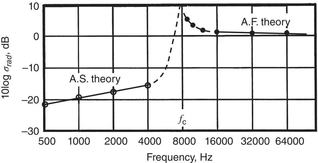
Refer to the panel in Example 12.8. Assume that the partition panel is made of steel (density = 7700 kg/m³) with internal critical damping ratio δ = 0.01 (1%). Plot 10log radiation efficiency σ_rad against log frequency f, where R_rad = ρcA_p σ_rad is the radiation resistance, A_p is area of panel, ρ = air density, c = speed of sound in air.

SOLUTION

The radiation efficiency σ_rad is calculated as follows:

‐ Panel radiation efficiency below coincidence:

where λ_c = coincidence wavelength = 343/8000 = 0.042 m, P = panel perimeter = 2(0.91+1.22) = 4.26 m, and A_p = panel area = 0.91×1.22 = 1.11 m².

If f/f_c = 1/16 (i.e. f = 500 Hz, assuming f_c = 8000 Hz):

Thus, 10 log σ_rad = 10log(0.0082) ≈ −21 dB. This calculation is repeated at f/f_c = 1/8, 1/4, and 1/2 which gives 10log σ_rad = −19.5, −18.0, and −16.5 dB, respectively.

‐ Panel radiation efficiency above coincidence:

At 16000 Hz, f/f_c = 2, σ_rad = . Thus, 10log σ_rad = 1.5 dB. The calculation is repeated at 9000 Hz, 10000 Hz and 12000 Hz which gives 10log σ_rad = 4.7 dB, 3.5 dB, and 2.3 dB, respectively.

If f →∞, σ_rad →1 and 10log σ_rad = 0. The results are plotted in Figure 12.21.

EXAMPLE 12.10

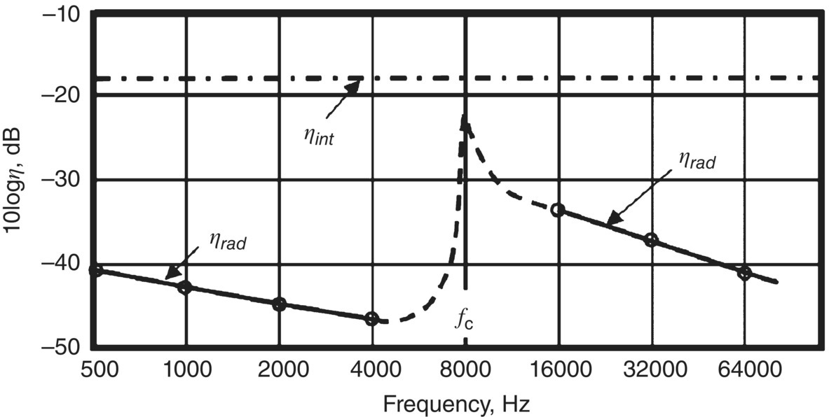
Consider the partition panel in Example 12.8 again. Plot 10log radiation loss factor ƞ_rad against log frequency, f.

Plot 10log ƞ_int on the same figure. Note ƞ_rad = (ρc/ωρ_s)σ_rad, where ρ_s is the panel surface density (mass/unit area).

SOLUTION

Radiation loss factor,

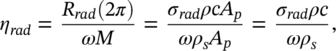
where ρ_s = panel surface density = 7700 kg/m³ × 0.0016 m, and ρ = air density = 1.23 kg/m³. Thus,

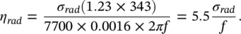
Then, 10log ƞ_rad = 7.4 + 10 log σ_rad – 10 log f.

Therefore, for f = 500 Hz we obtain 10log ƞ_rad = 7.4 −21 –10log(500) = −40.5 dB.

This calculation can be repeated at each frequency for which radiation efficiency data are available.

Now, η_int = 2δ = 2 × 0.01 = 0.02 (Remember that R = βM = ωηM = ω 2δM, where β is the energy loss factor).

Thus, 10log ƞ_int = 10 log (0.02) = −17 dB.

The results are plotted in Figure 12.22.

EXAMPLE 12.11

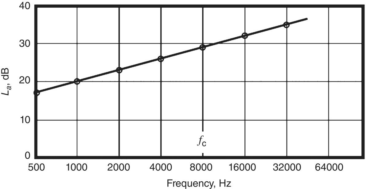
Vibration energy is fed into the partition panel in Example 12.8 through a point attachment of pipe carrying turbulent flow near one corner producing a force f_rms= 10 newton in each one‐octave band.

How much power is injected into the panel by this force?

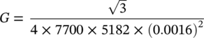
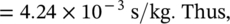
Assume the input point conductance G is given by  and that the input power .

Plot acceleration levels against 10 log f.

SOLUTION

Vibration Energy: Since f_rms = 10 newton, W_in = (10)² G,

where G is the assumed point input conductance for the plate 

[ for an infinite plate].

Note that for steel ρ_p = 7700 kg/m³ and c_l = 5182 m/s. Then,

L_a = 10 log (〈a²〉/g²) = 20 dB (in 1000 Hz band). We can easily calculate L_a at different frequencies (see Figure 12.23).

EXAMPLE 12.12

In Example 12.8, the storeroom is much too reverberant with a reverberation time of 1 second at all frequencies. Its volume is 85 m³.

Plot the space‐average sound pressure level in the cabin against log frequency caused by the force input in part Example 12.11. How much sound absorbing material should be added to the cabin walls, floor and ceiling to reduce the level by first 3 dB and then by 6 dB?

SOLUTION

We can write the following power flow equations using Eq. (12.42).

where W_dissP = power dissipated in panel, and W_dissR = power dissipated in room.

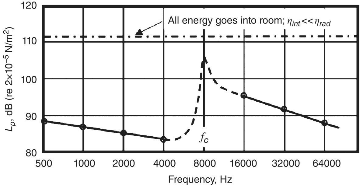
Also, the equations above in Section (d) and Eq. (12.42) and Figure 12.24b show that all the energy radiated into the room is absorbed in the room, i.e. W_rad = W_dissR.

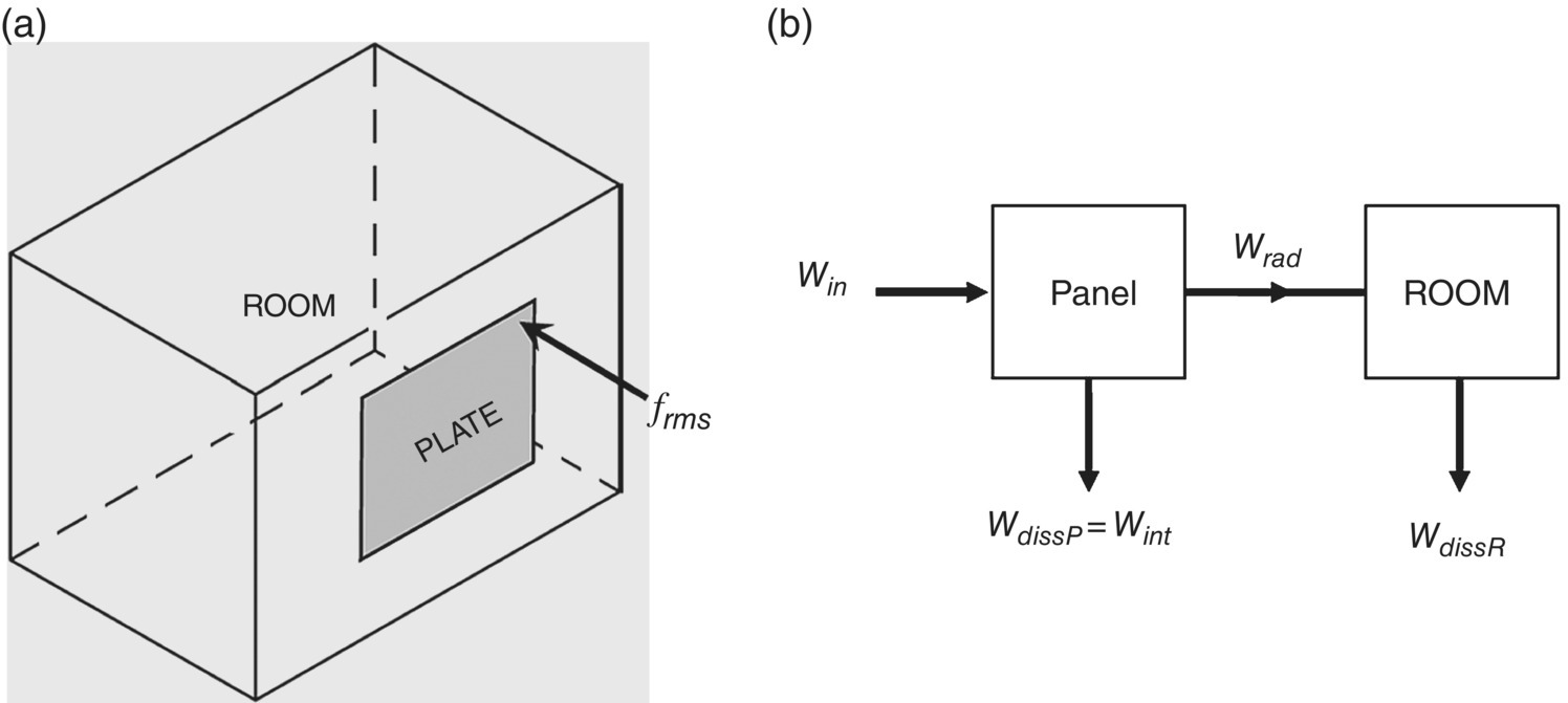
Energy density in room is p²/ρc² and total energy in room = p² V/ρc².

Thus, the rate at which energy is absorbed in room is

where β_room = ωη_room = 13.8/T_R, where T_R is room reverberation time.

Thus, the sound pressure level in room is

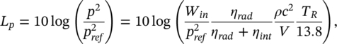
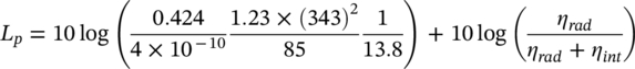
But we can read 10 log{η_rad /(η_rad +η_int)} from the curves in Example 12.10 (see Figure 12.22) by noting η_rad << η_int and simply taking the difference between the two curves. Thus, L_p is difference between two curves + 111 dB and the results are plotted in Figure 12.25. Note that if η_int were very small, η_int << η_rad and

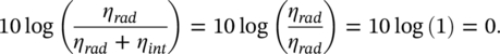
Then, there would be no power loss in the panel, the sound pressure level would be 111 dB in room.

To reduce the L_p by 3 dB we need to add some absorption area. We first need to calculate the existing absorption area in the room. This is related to the reverberation time T_R by Sabine’s formula (see Section 3.14.3 of this book).

Then, T_R = 0.161V/S , where V is room volume in m³ and S  = A, the absorption area in sabin (m²).

Now, V = 85 m³, T_R = 1 s, and the existing absorption area A₀ = 0.161×85/1 = 13.7 sabins (m²).

Hence the added absorption A₁ may now be calculated. The reduction in SPL, ΔL_p can be shown to be given by

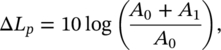
Hence 1+A₁/A₀ must be +2 and A₁ = A₀ = 13.7 sabins (m²).

Thus, total absorption at end of modification = 27.4 sabins (m²).

If we know what  is at any frequency, we can calculate the actual absorption area S  needed.

Analogously, if the desired reduction in sound pressure level is 6 dB, A₁ = 3A₀ = 41.1 sabins (m²), so the added absorption S  must be 27.4 sabins (m²).

12.4.3 Power Flow Between Coupled Systems

It has been shown that the power flow between coupled mode pairs is proportional to the modal energy difference, provided the coupling is weak and linear [40]. Scharton [46] and Ungar [26] have shown that the same result holds even if the coupling is not weak. Newland [42] has extended this result to include nonlinear coupling.

Ungar [26] explains simply how this result can be extended to consider the coupling between sets of modes. The same result can still be assumed to apply, provided either that the modes in each set are assumed to have approximately the same energy or that the coupling factors between the mode pairs are approximately the same.

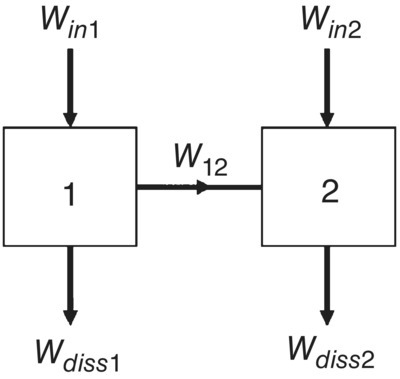
The power flow W₁₂ between systems l and 2 can be written as

(12.42)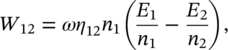

where two systems are considered (Figure 12.26). E₁ and E₂ are the total energies in systems 1 and 2 in the frequency band Δω and n₁ and n₂ are the modal densities (number of modes resonant in each system in the frequency band Δω considered). Thus, W₁₂ is the power flow in the frequency band Δω under consideration. The frequency ω is the center frequency in the band Δω. The result given by Eq. (12.42) may be used for several engineering applications, including airborne sound transmission through wall panels. We will confine ourselves to this application here. The modal energies given in Eq. (12.42) may be those of the air spaces (usually rooms) or the partitions or panels. Some discussion of the modal behavior of a panel is now in order.

12.4.4 Modal Behavior of Panel

The modes of a panel can be divided into two classes. Modes with natural frequencies above the critical coincidence frequency – and thus having bending‐wave speeds greater than the speed of sound in air – are termed AF. Modes with natural frequencies below the critical frequency – and thus having bending‐wave speeds less than the speed of sound – are termed AS. Further discussion about the panel modes is included in Section 3.16 of this book.

It can be shown theoretically [21, 24–28, 43] that the AF modes have a high‐radiation efficiency, while the AS modes have a low radiation efficiency. The AS modes may further be subdivided into two groups. AS modes, which have bending phase speeds in one edge direction greater than the speed of sound and bending phase speeds in the other edge direction less than the speed of sound, are termed “edge” or “strip” modes. AS modes which have bending phase speeds in both edge directions less than the speed of sound are termed “corner” or “piston” modes. Corner modes have lower radiation efficiencies than edge modes. The theoretical results for the radiation efficiency and classification of modes can also be given a simple physical explanation. Figure 3.27 in Chapter 3 shows a typical modal pattern in a simply‐supported panel or plate. The dotted lines represent panel nodes.

The modal vibration of a finite panel consists of standing waves. Each standing wave may be considered to consist of two pairs of bending waves traveling in opposite directions. Consider a mode which has bending wave phase speeds which are subsonic in directions parallel to both of its pairs of edges. In this case, the fluid will carry pressure waves which will travel faster than the panel bending waves, and the sound pressures created by the quarter‐wave cells (as shown in Figure 3.27a) will tend to cancel so that the effective volume source strength approaches zero everywhere except at the corners as shown. If a mode has a bending wave phase speed which is subsonic in a direction parallel to one pair of edges and supersonic in a direction parallel to the other pair, cancelation can only occur in one edge direction and for the mode shown in Figure 3.27b, the quarter‐wave cells shown will cancel everywhere except at the x‐edges. AF modes have bending waves which are supersonic in directions parallel to both pairs of edges. Then the fluid cannot produce pressure waves which will move fast enough to cause any cancelation, and the result is shown in Figure 3.27c.

Since AF modes radiate from the whole surface area of a panel, they are sometimes known as “surface” modes. With surface modes, the panel bending wavelength will always match the acoustic wavelength traced onto the panel surface by sound waves at some particular angle of incidence to the panel; consequently, surface modes have high radiation efficiency. This phenomenon does not happen for AS modes, the acoustic trace wavelength always being greater than the bending wavelength; AS modes have a low radiation efficiency.

At the critical coincidence frequency (when the panel bending wavelength equals the trace wavelength of grazing acoustic waves), the panel vibration amplitude is high [21, 22]. The radiation efficiency which is proportional to the radiation resistance is also high [21, 22]. Thus, at the critical coincidence frequency, the sound transmission is high and is due to modes resonant in a band centered at the frequency. Since the modes are resonant, the transmission can be reduced effectively in this region by increasing the internal damping of the panel.

Well below coincidence, because of their poor coupling with the fluid, the vibration amplitude of resonant modes is low, and the panel radiation efficiency is also low. In this region it is usually found that more sound is transmitted by modes which are not resonant in the frequency band under consideration. Since in such a band these modes are not vibrating at their resonance frequencies, they are little affected by internal damping. The contribution due to the non‐resonant modes gives rise to the well‐known “mass‐law” transmission. Just above the critical coincidence frequency, the panel vibration amplitude and the radiation efficiency are high and the transmission is still resonant. However, as the frequency is increased further, the internal damping usually tends to increase more rapidly than the radiation damping and the non‐resonant transmission becomes more important than the resonant transmission.

The relative importance of resonant and non‐resonant transmission, of course, depends upon the practical structure under consideration and upon the variation of internal and radiation resistance with frequency. The radiation resistance is normally increased with the addition of stiffeners, which will usually increase resonant transmission. An increase of internal damping which may be achieved in several ways, including the use of screwed or riveted structures or added damping material, will decrease resonant transmission and increase the importance of mass‐law transmission.

12.4.5 Use of SEA to Predict Sound Transmission Through Panels or Partitions

Lyon first used SEA to study the sound reduction of a rectangular enclosure with one flexible wall [45]. However he did not compare his results with experiment. White and Powell [50] used SEA to study the transmission of sound through double panels separated by an air space. Unfortunately, White and Powell restricted their theory to resonant transmission and did not allow for absorption in the air space between the panels or for the divergence from the room formula of the air space (cavity) modal density in the low‐frequency range (below f = c/2ℓ₂ or about 1700 Hz in their experiment, where ℓ₂ is the air gap width). It also appears that there is an error in their analysis, since they assume that the acoustic energy flow is proportional to the total energy difference between the systems instead of the modal energy difference.

The discussion which follows is based on work on the SEA sound transmission predictions and experiments on flat panels made by Crocker and his colleagues [27–30].

The transmission of sound through panels is usually measured in the laboratory using a transmission suite consisting of two rooms, as discussed in Section 12.7. The panel or partition under study is mounted between the two rooms. Consider the transmission suite shown in Figure 12.37. This may be considered to consist of three coupled systems, as shown schematically in Figure 12.27. System l is the transmission room; 2, the panel; 3, the receiving room. Under steady‐state conditions, the power flow balance for the three systems may be written: [21–24]

(12.43)

(12.44)

(12.45)

(12.46)

(12.47)

(12.48)

where W_in1, W_in2, and W_in3 are the rates of energy flow (in a frequency bandwidth of 1 rad/s, centered on ω) into systems 1, 2, and 3, respectively; W_diss1, W_diss2, and W_diss3 are the rates of internal dissipation of energy in systems 1, 2, and 3 (in a 1 rad/s band); E₁, E₂, and E₃ are the total energies of systems 1, 2, and 3 (in a 1 rad/s band), and n₁, n₂, and n₃ are the modal densities of each system (modes per radian per second); η₁, η₂, and η₃ are the internal loss factors of each system; η₁₂, η₁₃, and η₂₃ are coupling loss factors between systems l and 2, 1 and 3, and 2 and 3, respectively. The formulation so far in Section 12.4.4 is quite general and can be applied to any three coupled systems. Now it will be applied to the particular sound transmission case.

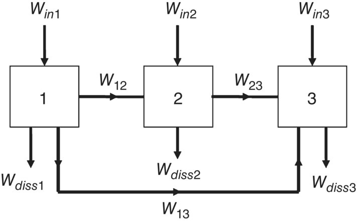
It is assumed that the panel is clamped between the transmission room (volume V₁) and the reception room (volume V₂) of the transmission suite. Reverberant sound is produced in the transmission room by a loudspeaker. In this case, the noise reduction (NR) NR = 10log(E₁ V₃/E₃ V₁); consequently, the sound transmission loss produced by the panel may be determined from Eqs. (12.43) to (12.48) with W_in2 = 0 and W_in3 = 0.

Putting W_in2 = 0 in Eq. (12.46) and also using the reciprocity relationship η₁₂ n₂ = η₂₁ n₁ [31], Eq. (12.49) is obtained:

(12.49)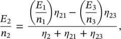

but η₂₁ = η₂₃ = η_rad (the panel radiation loss factor) and except at low frequency where the present theory does not apply, E₁/n₁ ≫ E₃/n₃; thus Eq. (12.49) becomes

(12.50)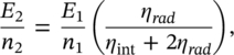

where η_int = η₂ is the internal damping loss factor of the panel. Putting W_in3 = 0 in Eq. (12.48) yields

(12.51)

The term E₁ η₂₃ represents the mass‐law or non‐resonant transmission since it occurs without the modes resonant in the frequency band under consideration being excited. The term E₂ η₂₃ represents the resonant transmission. Substituting Eq. (12.50) into Eq. (12.51) gives

(12.52)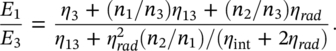

Equation (12.52) gives the ratio of total energies in the transmission and receiving rooms. The parameters η₁₃, η_rad and η₃ can be evaluated from the following equations:

(12.53)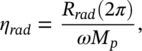

where M_p is the panel mass, and the panel radiation resistance to half space R_rad(2π) is given by Maidanik [39]. It should be noted that the expressions given for R_rad(2π) for f < f_c and f > f_c given in Ref. [26] contain printing errors, but the correct expressions are given in Ref. [22], where, unfortunately, the expression for f = f_c contains a printing error.

The coupling loss factor η₁₃ due to non‐resonant mass law transmission is obtained from (see Section 12.2.1)

(12.54)

where TL_rand, is the random incidence mass‐law TL value for the second system (the panel). The value of TL_rand given by Eq. (12.21) can be used in Eq. (12.54). Finally,

(12.55)

where T₃ is the reverberation time in system 3.

If Eqs. (12.53)–(12.55) are evaluated and a value for η_int is chosen, or else measured by experiment, then the NR = 10 log(E₁ V₃/E₃ V₁) can be found from Eq. (12.53):

(12.56)

where the room (n₁ and n₃) and panel (n₂) modal densities are (see Section 12.4.2)

(12.57a)

(12.57b)

(12.57c)

where S, h, c_l are the panel area, thickness, and longitudinal wave speed. The TL of the panel is then

(12.58a)

The response of the panel relative to mass law is easily derived from Eq. (12.50). We first assume that the sound field in the transmission room is reverberant, so that the total energy in a 1 Hz bandwidth E₁ = Sρ₁ V₁/(ρc²) and the total panel energy in a 1 Hz bandwidth E₂ = M_p S_a/ω². We then also substitute the modal density of the transmission room n₁(ω) = V₁ ω²/(2π² c³), the modal density of the panel n₂(ω) =  A_p/(2πhc_L), and the critical frequency f_c =  c²/(πhc_L), into Eq. (12.50). Finally, we assume that if the panel were to respond as a limp mass, the response would be S_aml/S_pω = 1/ρ²_s, where S_pω is the spectral density of the pressure at the panel wall surface. Neglecting panel motion, S_pω = 2S_p1, since there is pressure doubling for each wave arriving at the panel surface, although at any instant only half the waves are traveling toward the panel. Thus, S_am1/S_p1 = 2/ρ²_s and with this final substitution, Eq. (12.58b) is obtained. See Ref. [22].

(12.58b)

where S_a, S_aml. are the spectral densities of the acceleration of the panel given by the present theory and given by mass law theory, respectively; η_int is the panel internal loss factor; ρ and ρ_s are the air density and panel surface density.

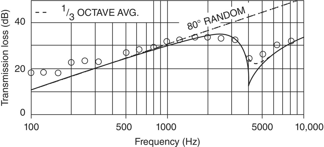
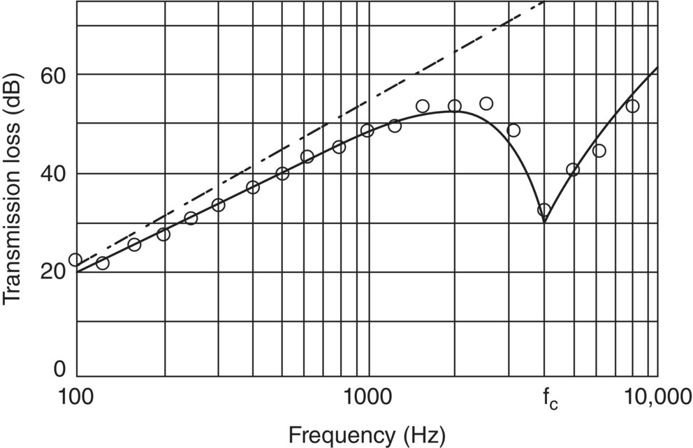
Figure 12.28 shows a comparison [27, 28] between the measured TL of a single wall aluminum panel and that calculated from Eqs. (12.56) and (12.58a). The panel studied was 1/8 in. (3.175 mm) thick and measured 61 in. by 77.5 in. (1.55 m by 1.97 m). The values of η_int used in the predictions was 0.005. Measured values of η_int varied between 0.005 and 0.01 throughout the frequency range 100–10 000 Hz [27, 28]. The agreement is good with two exceptions. At low frequency f < 400 Hz, the disagreement is thought to be caused by room‐panel modal coupling effects. Just below the critical coincidence frequency, agreement between theory and experiment is considerably improved if the radiation resistance R_rad (2π) is assumed to be twice the value for a simply supported panel for f < f_c. This is a good assumption to make since the panel edge conditions were intended to be clamped and R_rad (2π) for a clamped panel is twice that for a simply supported panel.

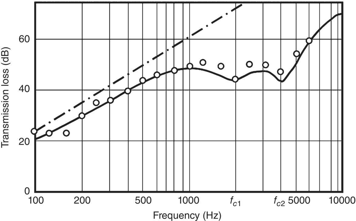
Theory for a double‐partition system can also be derived [28, 30]. If the double partition consists of two independent panels separated by an air cavity, then the theoretical model shown in Figure 12.27 must be extended to include five oscillators (room‐panel‐cavity‐panel‐room). The development is similar to that given in Eqs. (12.43) through (12.48), although now five power flow balance equations are obtained instead of the three in Eqs. (12.43) through (12.48). Complete details of the theory are given in Refs. [21, 23, 26]. Figure 12.29 gives an example of a comparison [28, 30] between the measured TL and that predicted by the SEA theory for double panels just discussed. Each panel was 1/8 in. (3.175 mm) thick with the same length and width as the single panel in Figure 12.28. The upper broken curve in Figure 12.29 shows the predicted TL assuming non‐resonant (or mass‐law) transmission through each panel only. This is the result to be expected if each panel became limp (that is, if each panel had no stiffness or damping but maintained the same mass per unit area as the 1/8 in. [3.175 mm] thick aluminum panels).

It is observed, when comparing Figures 12.28 and 12.29, that the double‐panel system TL curve is steeper than the corresponding one for the single panel. Not only is the double‐panel curve everywhere more than 6 dB above the single‐panel curve (6 dB increase would be expected for a single panel of twice the mass), but the slope is greater for the double panel. Below the critical coincidence frequency, the TL of the double panel increases about 9 dB per doubling of frequency compared with 6 dB for the single panel.

Figure 12.30 shows measured and predicted results for a double‐panel system with panels of the same dimensions as in Figure 12.28, except the panels have different thicknesses (1/4 in [6.350 mm] and 1/8 in. [3.175 mm]). Two dips in the TL are now seen at 2000 and 4000 Hz. The dips are now not as sharp as in Figures 12.28 or 12.29.

The measured acceleration response of the panel (compared with the response predicted by mass law), is given in Figure 12.31. The measured response is compared with the response predicted by Eq. (12.58b) for η_int = 0.005. The agreement is good except at low frequency. The low frequency disagreement is again much reduced if R_rad (2π) is assumed to be twice that for a simply‐supported panel for f < f_c. Since all the panels measured had clamped edges, this would seem to be a reasonable assumption. The high frequency disagreement is removed in Figure 12.31, if η_int = 0.01 for f > f_c. This value is closer to the experimental result for f > f_c.

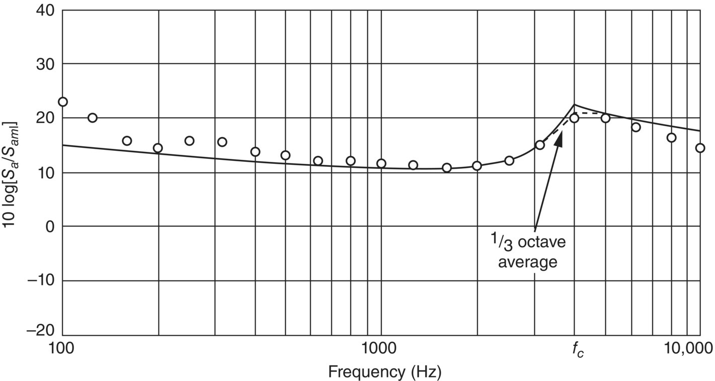
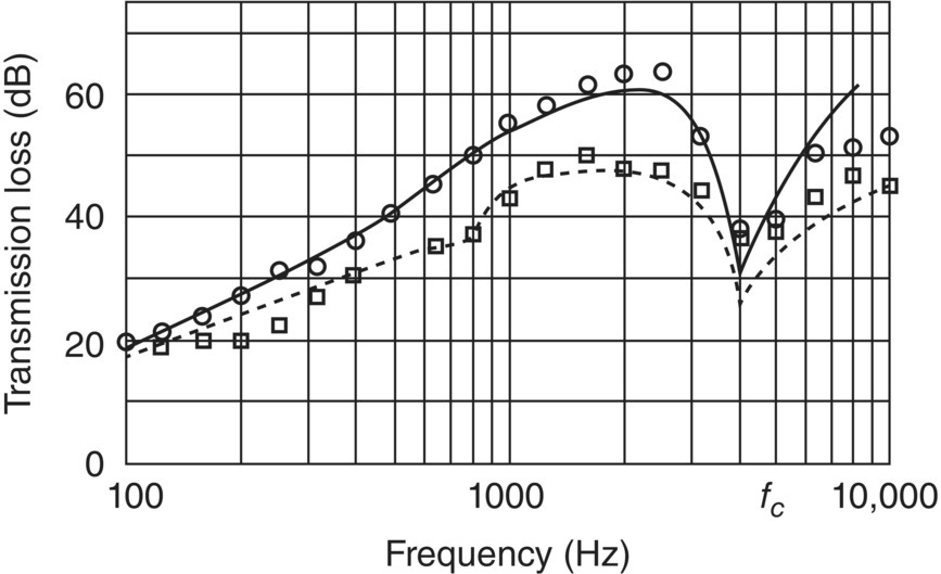
Figure 12.32 shows experimental and theoretical results for a 1/8 in. (3.18 mm) thick aluminum double‐panel system with and without tie beams [30]. The experimental results were obtained both for the case where the panels were connected together by 50 steel coupling ties and for the case where they were independent. The ties were each 2.8 in. (7.11 cm) long, 1 in. (2.54 cm) wide and 0.027 in. (0.69 mm) thick. It is observed that, although the independent double panel is identical to that given in Figure 12.29, the transmission loss is higher in Figure 12.32 above 500 Hz, presumably due to higher internal panel damping. A theoretical prediction for this case shown in Figure 12.32 with η_int = 0.005 for f < 800 Hz and η_int = 0.02 for f > 800 Hz is seen to give good agreement with the measurements.

12.4.6 Design of Enclosures Using SEA

Airborne noise transmission into enclosures is of interest to designers of operator enclosures in factories, cabs for trucks, cabins for aircraft and farm tractors, ships and even satellite enclosures in spacecraft. In this section of the chapter, such an enclosure is modeled both theoretically and experimentally as a rectangular steel box immersed in a diffuse reverberant sound field [51–55]. The box is structurally isolated from the field and the sound attenuation is determined. The effects of small apertures in the box wall are also examined [55, 56]. SEA has been used for the theoretical analysis and the experimental measurements were performed while the box was being excited by broadband random noise suspended inside a reverberation chamber [55, 56].

The SEA prediction scheme incorporated the presence of small apertures of regular geometry in one panel and acoustical absorbing material inside the box. The attenuation was measured in one‐third octave bandwidths whose center frequencies ranged from 63 Hz to 20 kHz. From these results, conclusions can be drawn as to the best ways of maximizing the NR of cabin enclosures [56, 57].

For the purposes of the analysis, the system is separated into eight individual elements, as shown in Figure 12.33a. The box itself is comprised of elements 2 through 7, these being the steel panels which are the sides of the box, while the exterior acoustical space, which is the reverberation room is element 1 and the interior box cavity is element 8.

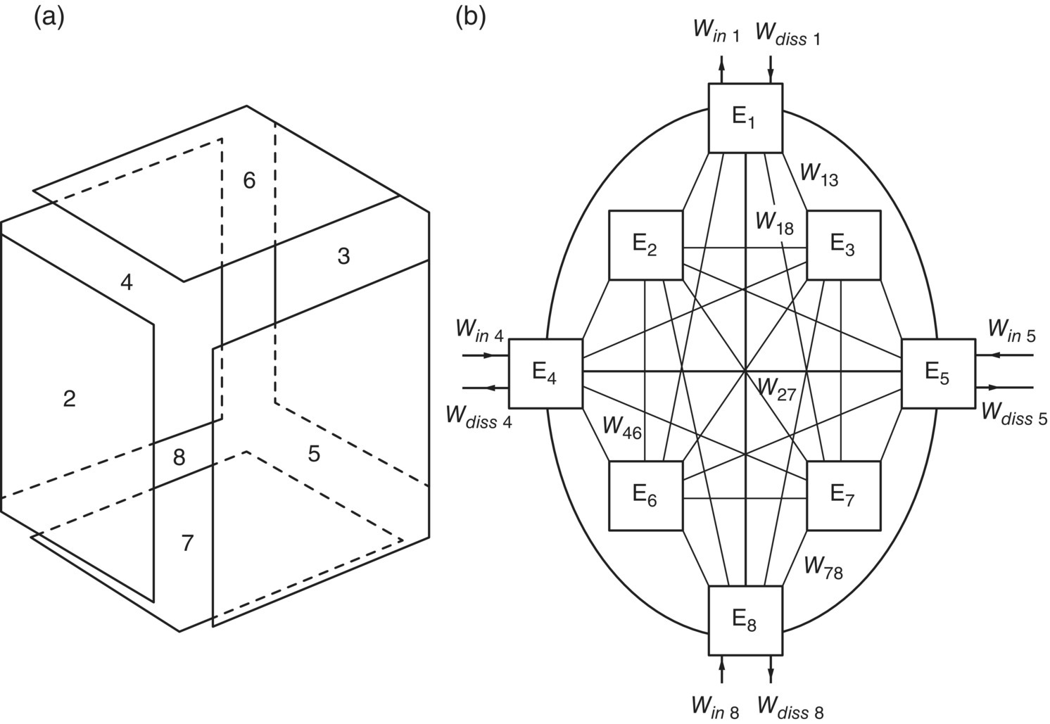
A schematic power flow diagram is shown in Figure 12.33b. The figure shows each element coupled to every other element and to certain elements is attributed an input power. In reality, panels which are not contiguous are not (directly) coupled and for the purposes of the NR prediction, only element 1 receives any input power. Since only airborne sound transmission is being investigated. The box is assumed to receive no direct mechanical excitation [54].

An eight element system requires an 8 × 8 matrix equation to model the power flow [54]. At a center radian frequency of ω and for an arbitrary bandwidth Δω, the first power balance equation for power input to element 1 may be written:

In terms of the modal energies E/n in that bandwidth:

where ω = 2πf.

Seven other similar power balance equations may be written for the seven other elements. The entire system of power balance equations over a bandwidth Δf may be solved so that the modal energies in each system may be obtained by a pre‐knowledge of the power inputs to each element. In the case of the cab model, W_in2, W_in3, W_in4, …, and W_in8 are all assumed equal to zero, while W_in1 represents the acoustic power flow into the reverberation room from a noise source.

The resonant coupling loss factors are represented in the matrix equation as ŋ_JI where I is the panel number and J is the acoustical space number (the loss from the panel to the room/box cavity) and ŋ_IJ (the loss from the room/box cavity to the panel).

Included in the non‐resonant loss factor is the effect of small holes in the panels. These holes represent direct transmission paths between the outside and the inside of the box, and the loss factor due to these may be calculated and combined with the mass law loss factor.

The power flow equations may be evaluated and solved for a variety of system configurations. The basic calculation is for a completely sealed (no holes) empty box, and thereafter the effect of absorbing material in the box, circular apertures and rectangular apertures may be considered. Each of these situations has been modeled and compared with experimental measurements [54].

The sound pressure level difference outside to inside of the box, sometimes known as NR, is termed attenuation in this section of this chapter. The sound pressure level (L_p) in the box is evaluated, and the attenuation may thus be calculated:

or

where N₁, V₁, E^m₁, and N₈, V₈, E^m₈ are the mode counts, volumes and modal energies of the exterior and interior air space cavities. The attenuation is thus calculated for each bandwidth at the center frequency f, and is best displayed when plotted against log(f). The experimental values of attenuation, measured in one‐third octave bands, are then plotted on the same graph as the theoretical curve for comparison.

Various methods of deriving the sound transmission coefficient of an aperture in a rigid wall have been presented in the literature. For the purposes of this chapter, the transmission coefficient for the aperture, a, derived by Ingerslev and Nielsen [59] and referred to in Mulholland and Parbrook [58] was chosen for its simplicity.

In Figure 12.34a, the predicted and measured results are compared for the case of a sealed box (with no apertures) with 1.2 m² absorbing material inside. The shape of the theoretical curve is to be expected; a smooth rise through the low and middle frequencies according to the so‐called mass law transmission (see Section 12.2.1) which dominates in this frequency range. As the frequency approaches the critical coincidence frequency, about 8000 Hz, a rapid drop occurs due to the increased vibration response and radiation efficiencies of the panels. Above this frequency, the attenuation increases, since it is in the frequency range where the panel mass and damping control the transmission loss [53].

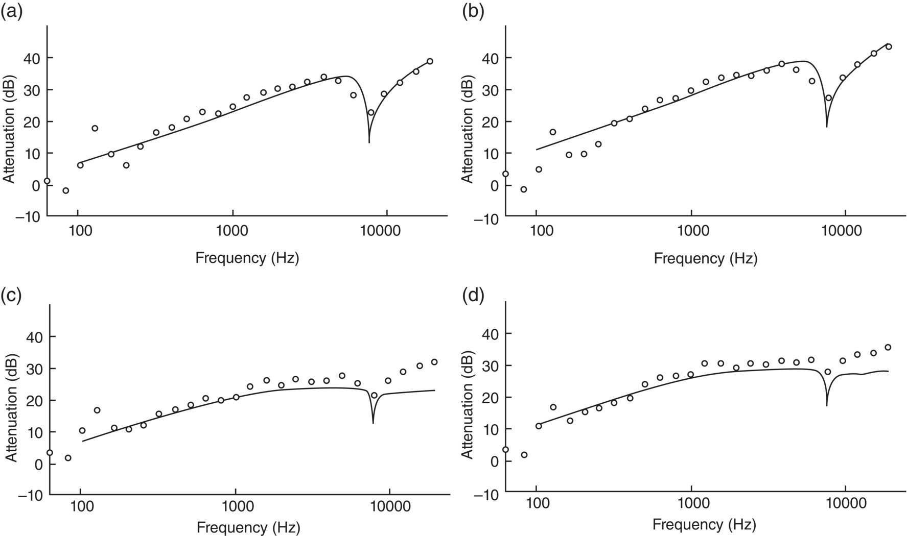
The agreement between experiment and theory is good throughout much of the frequency range. Exceptions occur at low frequencies, below about 200 Hz, and at the critical coincidence frequency. The latter anomaly may be attributed to the fact that the theoretical curve is calculated using frequency bandwidths of 100 Hz, while the experimental values were measured in one‐third octave bandwidths.

In Figure 12.34b the predicted and measured results are compared for the case of a sealed box containing 3.5 m² absorbing material [53, 54]. All comments pertaining to the previous figure also apply directly to this one. The major difference between Figure 12.34c and d is caused by the increased amount of absorbing material in the box; the attenuation is approximately 4 dB higher throughout the entire frequency range as would be predicted from 10log(3.5/1.2).

Figure 12.34c shows the effect of a circular aperture in one panel and compares the experimental data with predicted values calculated using the value for the aperture transmission coefficient, α, given in Ref. [54]. The aperture has a diameter of 0.035 m and the box contains 1.2 m² of absorbing material. Comparison with Figure 12.34c of both the predicted and measured curves, shows how the aperture only affects the attenuation in the middle and high frequency range. Below a frequency of about 500 Hz, the mass law transmission is dominant over the relatively poor transmission of sound by the aperture. Above this frequency, the aperture contributes more and more to the overall transmission as the frequency increases. However, at the critical coincidence frequency the attenuation is the same as that of a sealed box because the efficiently radiating panels dominate in the transmission behavior.

The measured results agree with the theory up to about 1000 Hz. The discrepancies at the lowest frequencies are due to the reasons described previously. It is questionable whether the extreme low frequency theoretical results should be presented, since their meaning is unclear, at least below 163 Hz, which is the lowest frequency at which a mode can exist in the box air cavity. Above 1000 Hz, which corresponds to an aperture ka value of about 0.4, (where a is the aperture radius and k is the wave number) the predicted attenuation is consistently lower than the measured attenuation. As expected, the aperture transmission theory breaks down at high values of ka, and the disagreement becomes more apparent as the frequency increases. The model predicts more efficient transmission by this aperture than is actually observed [53].

Figure 12.34d compares the measured and predicted attenuation of the steel box which has a circular aperture (of diameter 0.035 m) and contains 3.5 m² of absorbing material. In the theoretical predictions, the aperture transmission coefficient a given in Ref. [53] was used. In comparing these results with Figure 12.34b the attenuation is found to be increased by about 4 dB at every frequency. This is the same result as obtained for the sealed box (compare Figure 12.34a and b). Comparison with Figure 12.34b again shows how the aperture only affects the attenuation in the middle and high frequency ranges. As in the case of Figure 12.34b the predictions become less accurate at high frequencies [53, 54].

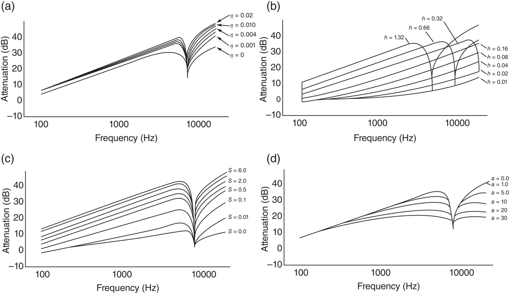
A number of parameters of the enclosure are varied while the others are kept constant. Figures 12.35a–d show the effects of varying panel damping, thickness, internal sound absorption area, and aperture radius in the idealized truck cab enclosure while each of these other variables are kept constant.

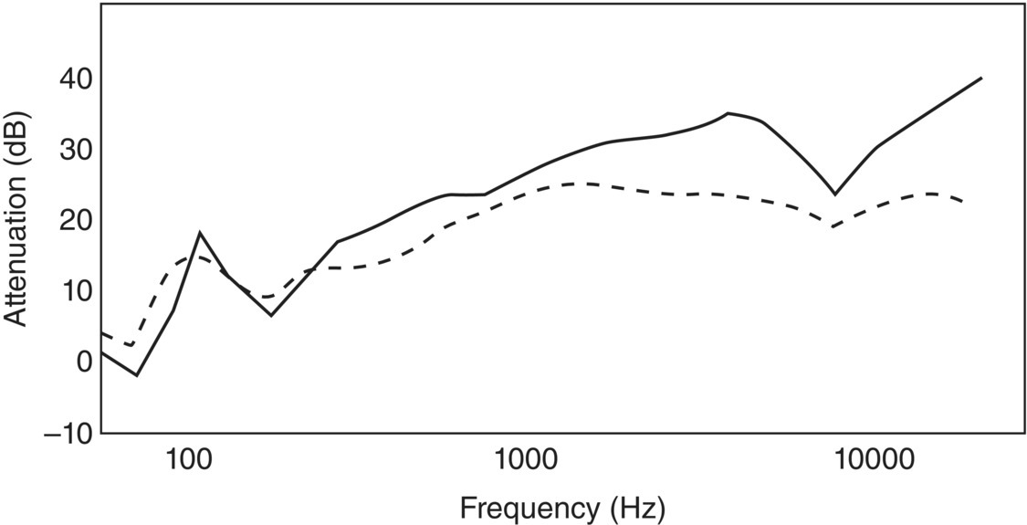
Finally, Figure 12.36 shows the difference in experimental results between the attenuation of an idealized cab enclosure with the leaks between panels unsealed and sealed with clay. The attenuation is defined as the difference in space‐averaged sound pressure levels outside and inside the enclosure.

12.4.7 Optimization of Enclosure Attenuation

As seen in the earlier analysis, the sound power transmission into the enclosure has a complicated relationship with the different parameters of the system. These effects vary widely with frequency. If the system is subjected to an external diffuse reverberant sound field, it is convenient to take frequency averages of the attenuation over the whole frequency range. For an effective design of the system to minimize the overall attenuation level, all parameters must be considered simultaneously by performing the optimization. The constrained optimization method was used to consider the bounds on the parameters. The design variables for the optimization problem were set with x₁ as the aperture radius in m, x₂ as the panel thickness in m, x₃ as the absorption area in m² and x₄ as the panel density in kg/m³. The optimization problem can be described as follows:

The initial design variables were taken as x₁ = 0.01 m, x₂ = 0.00159 m, x₃ = 0.5 m², and x₄ = 7790 kg/m³. The Constrained Optimization Module of MATLAB version 5.2 was used for the optimization. A typical configuration x₀ as described above was used as an initial estimate for the optimization. This configuration gives after optimization, aperture radius x₁ = 0.005 m, panel thickness x₂ = 0.0011 m, absorption area x₃ = 3 m² and panel density x₄ = 8000 kg/m³.

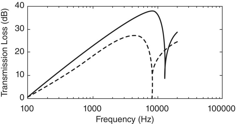
The effect of the optimized design on the attenuation is shown in Figure 12.37 [57]. There is a substantial increase in attenuation over the entire frequency range. It shows the importance of considering all the parameters simultaneously for optimization. Further parametric studies of the transmission loss of panels are discussed in a recent paper on single and double-walled plates with absorbing materials [60].

12.4.8 SEA Computer Codes

In the simple calculations presented in Examples 12.8 to 12.12, only hand calculations are needed and these can be performed on the “back of an envelope.” This illustrates the beauty and simplicity of SEA. However, for the more complicated sound transmission problems in Sections 12.4.5–12.4.7, computer software codes were written. Such codes allowed more complicated equations to be used, but also for mechanical and acoustical properties to be varied so as to examine their effects on the SEA predictions.

In the 1980s commercial software codes became available such as AutoSEA marketed by Vibro‐Acoustic Sciences. This code has been updated as AutoSEA2. Hybrid codes have now been developed, in which SEA is coupled to finite element method (FEM) or BEM. One such code known as VA One was developed after Vibro‐Acoustic Sciences was sold to ESI. A new FEM/SEA code, Wave6 is now marketed by Dassault and is used by a wide range of industries. Other computer software codes available for SEA of complex sound and vibration problems are GSSEA‐Light marketed by Gothenburg Sound AB and Seam marketed by Altair.