Sound Transmission Theory for Single Panels

12.2.1 Mass‐Law Transmission Loss

We will consider the case of a plane sound wave incident on a partition. For simplicity, we shall assume that the partition is thin (in wavelengths) and infinite in extent. For convenience, we assume that the x‐ and y‐axes are in the plane of the paper (see Figure 12.1) and that the direction of propagation of the wave is in the x‐y plane, so that there is no variation in the z‐direction (perpendicular to the paper).

Thus, the three‐dimensional wave equation (see Eq. (3.29)) reduces to the two‐dimensional wave equation:

(12.1)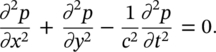

We may assume plane waves p_i, p_r, p_t, incident, reflected, and transmitted by the panel (Figure 12.1b). If the panel stiffness and damping are negligible, it will act like a limp mass, and the panel will be forced into motion. If we assume that the incident wave has a frequency f, then the panel will be forced into vibration at this frequency, and the reflected and transmitted waves will also have the same frequency. The wavelengths and wave numbers of the incident, reflected, and transmitted waves must be the same, provided the fluid medium is the same on each side of the panel. By Snell’s law, the angles of incidence, reflection, and transmission will also be the same (equal to θ). Provided the fluid remains in contact with the surface of the panel everywhere, the trace wavelength of the vibration on the panel λ_T = λ/sinθ, where λ is the wavelength in the fluid.

Equations for the plane waves in the fluid which satisfy Eq. (12.1) are given by

(12.2a)

(12.2b)

(12.2c)

The amplitudes of the waves A₁, B₁, and A₂ are shown as complex quantities since the waves are not necessarily in phase with each other (see Chapter 3). The wave number components k_x and k_y, in the x‐ and y‐ directions are related to the wave number k by

(12.3a)

and

(12.3b)

See Figure 12.1a, which shows the situation for the incident wave. Squaring Eqs. (12.3a) and (12.3b) and adding gives

(12.4)

This result can also be seen from Figure 12.1a or by substituting any of the Eqs. (12.2a), (12.2b), or (12.2c) into Eq. (12.1) and remembering that k = ω/c.

The ratio of the square of the amplitude of the transmitted wave compared to that of the incident wave is the quantity which is of most interest, since it tells us the fraction of energy transmitted by the partition. This fraction is called the transmission coefficient, τ = ∣ A₂∣²/∣ A₁∣² and may be determined using the following two conditions:

1. The acoustic particle velocity normal to the panel surface on each side of the panel must equal the panel velocity v_w at each point.
2. The total pressure acting on the panel equals the mass per unit area times the acceleration jωv_w at each point.

The first condition leads to

(12.5)

If the panel is very thin, then the pressures p_i, p_r, and p_t near the panel surface are given by putting x = 0 in Eqs. (12.2a)–(12.2c) which, when substituted into Eq. (12.5), gives

(12.6)

The second condition gives

(12.7)

Neglecting stiffness K and damping R in the wall, we may put the wall impedance per unit area, Z_w = jωM, where M is the mass per unit area of the wall. The pressures in Eq. (12.7) again must be evaluated at x = 0. Substituting Eqs. (12.2a)–(12.2c) into (12.7), with x = 0, and using v_w = (p_t/ρc)cos θ from Eq. (12.5), gives

(12.8)

Substituting Eq. (12.6) into (12.8), and eliminating B₁, gives

(12.9)

The ratio of the intensity of the incident and the transmitted waves is

(12.10)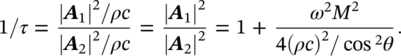

The quantity, τ in Eq. (12.10) is known as the sound transmission coefficient. We define a logarithmic quantity, the transmission loss (TL), to be

(12.11a)

(12.11b)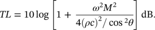

Note that TL, the transmission loss in decibels, is sometimes known as the sound reduction index in Europe and in International Organization for Standardization (ISO) standards (see Section 12.6). The logarithm of 1/τ instead of τ is used in order to obtain positive numbers.

We note that, according to this theory, when a wave approaches the panel at grazing incidence (parallel to its surface), TL → 10 log(1) → 0 because cos θ → 0 and the wave is transmitted through the panel without any attenuation; however, this is an unusual situation in real cases. If a wave approaches the panel in a direction normal to its surface, the transmission loss is maximum. Unless we consider very light panels and very low frequencies, or panels immersed in a fluid medium having a high value of ρc then

and

(12.12)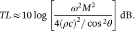

This result is known as the mass law. We note that the TL is governed by the mass per unit area, M, of the panel. For a fixed angle of incidence θ, if the frequency, ω = 2πf, is kept constant, then each time the mass per unit area of the wall is doubled, the TL increases by 10 log (4) = 20(0.301) ≈ 6 dB. For a fixed angle of incidence and fixed mass per unit area M, likewise the TL increases by 6 dB for each doubling of frequency (octave) (see Figure 12.2). We have probably all experienced these phenomena in our everyday lives: we know that (i) thick massive walls have a much better TL than thin ones, and (ii) we hear the low notes of music transmitted through walls in buildings much better than the high notes.

EXAMPLE 12.1

Determine the transmission loss for normal incidence at 1000 Hz of a single panel made of aluminum 3 mm‐thick and density 2700 kg/m³.

SOLUTION

The mass per unit area of the panel is M = 2700 × 3 × 10⁻³ = 8.1 kg/m². If we substitute M, ω = 2πf = 2π(1000) = 6283 rad/s, and θ = 0° into Eq. (12.12), we obtain the TL for normal incidence: TL = 20 log [(6283 × 8.1)/(2 × 1.18 × 344)] = 35.9 dB.

So far in this section, it has been assumed that the panel behaves as a limp mass. It is difficult to include the effects of plate stiffness and damping exactly, but these may be included approximately as follows. We will assume that the panel stiffness and damping can be distributed uniformly over the surface area, so that Z_w in Eq. (12.7) is replaced by jωM + R + K/jω instead of jωM. Here, R and K are the damping and stiffness coefficients per unit area. Then instead of Eq. (12.11b) we obtain

(12.13)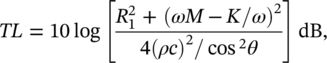

where R₁² = (R + 2ρc/cos θ)².

Equation (12.13) is plotted in Figure 12.3. At very low frequency, the sound transmission is controlled by the panel stiffness. As the frequency is increased, the panel resonance frequency ω_n is reached, and if the damping R is zero, the panel becomes transparent to sound, and TL = 0. As the frequency is increased still further, the TL is dominated by the panel mass (inertia), and of course Eq. (12.13) is equivalent to Eq. (12.12) at high frequency. This simple theory does not predict the coincidence effect predicted by more sophisticated theories (see Section 12.2.3). The effect of higher panel resonances is also not predicted by the theory because the theoretical model is an equivalent single‐degree‐of‐freedom system.

For most building elements, the first panel resonance generally occurs below the practical frequency range of interest, so its effect can be omitted. The TL in the vicinity of this resonance frequency depends strongly upon the panel damping and the characteristics of the incident sound field, both of which are very difficult to estimate. However, in order to improve the attenuation of a panel, the damping should be as large as practical. Also, so far, the attenuation of a panel to sound at only one angle of incidence has been considered. In most practical cases, sound waves strike a panel from many angles simultaneously (random incidence). Figure 12.4 shows the TL of a partition, including the effect of higher order panel resonances and the coincidence effect (see Section 12.2.3). Figure 12.4 is deduced partly from theoretical and experimental considerations.

12.2.2 Random Incidence Transmission Loss

In practice, sound will strike the partition from many angles simultaneously. Thus, some averaging over the angle of incidence of the theoretical results, such as Eq. (12.11) or Eq. (12.12), is necessary in order to predict the partition transmission loss for this case.

If we consider waves to approach the hemispherical area shown in Figure 12.5 with equal probability, we could choose a limiting angle θ′ = 60° to give an approximate average transmission loss for the waves approaching the surface dS. This is because when θ′ = 60°, half of the surface area of the hemisphere is above this angular element dA, and half is below. If we substitute θ = 0° into Eq. (12.12), we obtain the TL for normal incidence:

(12.14)

Then with θ = 60° in Eq. (12.12), we obtain an estimate for the TL for random incidence:

(12.15)

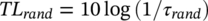
(12.16)

since cos 60° = 1/2 and 10 log (1/2)² = 6 dB. This result for TL_rand in Eq. (12.15), agrees fairly well with experimental results.

A more rigorous way of estimating TL for random incidence sound is to find the average value of the transmission coefficient τ_rand, averaged properly over all angles, using Eq. (12.10) and Figure 12.5. Waves approaching the surface of the wall partition at angle θ, only “see” a projected area dS cos θ. The transmission coefficient depends on angle θ and, thus, in the averaging process must be “weighted” by cos θ. The average transmission coefficient for random incidence τ_rand is thus

(12.17)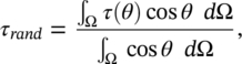

where Ω is the solid angle.

Since the differential of the solid angle dΩ = sin θ dθ dϕ, we may rewrite Eq. (12.17) as

(12.18)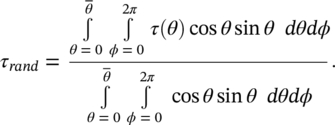

For those of us unfamiliar with the use of solid angles, we may care to consider the waves traveling through the small area dA. By putting r = 1, dA = sinθ dθ dϕ and after weighting τ(θ) by cos θ and averaging over all angles, we arrive again at Eq. (12.18). Using Eq. (12.10) we can write

(12.19)

where a = ωM/2ρc. However, since d(sin² θ) = 2sin θcos θ dθ and d(1 + a²cos² θ) = −2a²cos θsin θdθ, we may rewrite Eq. (12.18) as

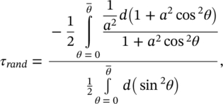
(12.20)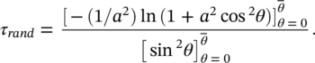

If we average over all angles  = 90°, , and . Thus,

(12.21)

and since a = ωM/2ρc, we see from Eq. (12.14) that TL₀ = 10 log(a²). Thus,

(12.22a)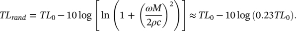

We see as we saw in Eq. (12.16), that the random incidence TL is again predicted to be less than the TL at normal incidence. This is to be expected since the random incidence TL is heavily weighted by waves, for which θ > 0° and in which TL < TL₀.

It is found that Eq. (12.22a) does not agree well with experimental results, and it is normal practice to argue that we should use θ = 78° instead of 90°, in order to obtain better agreement between theory and experiment. The result of averaging τ(θ) over all angles of incidence from normal (0°) to 78°, using the two Eqs. (12.19) and TL = 10log[1/τ(θ)], is usually known as the field‐incidence, mass‐law transmission loss (TL_field). The integration is performed up to θ = 78° instead of 90° to obtain better agreement with experiments. Several reasons are usually quoted to justify this, including (i) the finite size of the partition, (ii) the effect of the test facility and the possible paucity of room modes which would give rise to sound waves near grazing incidence, and (iii) damping effects in the partition for near grazing incidence waves. It should be noted that some authors have used other values of θ, e.g. 80° or 81° [6]. Figure 12.6 shows a nondimensionalized plot of the mass‐law transmission loss of a limp‐wall for normal incidence (θ = 0°), several other values of incidence (45°, 60°, and 78°), field incidence (θ = 78°), and random incidence (θ = 90°).

The transmission loss curves given in Figure 12.6 are only valid in the mass‐controlled frequency region of a partition (see Figure 12.4). However, they do illustrate the most important features of the TL of a partition: the fact that the TL increases as the mass per unit area or the frequency of the incident sound are increased. It is noted that a TL somewhat less than that predicted by the mass‐law portion of the curve should be expected at the lowest panel resonance in the damping‐controlled frequency region. Also, it is seen that the highest TL is for sound approaching at normal incidence. For prediction purposes, it is best to use the field‐incidence TL curve if it is expected that the sound approaching the partition comes from many directions instantaneously. This is the normal case in practice. One exception might be, for example, the noise of traffic reaching the windows and walls of the upper stories of high‐rise buildings. In this case, the sound would be much nearer to grazing incidence, and a TL lower than the free‐field TL would result.

We see from Figure 12.6 that approximately

(12.22b)

Often the equation

(12.22c)

is used as an empirical fit for Eq. (12.21) or (12.22b). Here, M is the surface density, f is the frequency in Hz, C = 47 if the units of ρ_s are kg/m² and C = 34 if the units are lb/ft². Equation (12.22b) may be compared with Eq. (12.16). Again it should be emphasized that Eq. (12.22c) does not include the effects of sound transmitted in the frequency region in which coincidence occurs (see Figure 12.4).

EXAMPLE 12.2

Calculate the TL for normal and field incidence at 500 Hz of a brick wall with a mass per unit area of 415 kg/m².

SOLUTION

We have that ω = 2π(500) = 3142 rad/s. From Eq. (12.14) we obtain that for normal incidence TL₀ = 20log[3142 × 415/(2 × 1.18 × 344)] = 64.1 dB.

For field incidence we may use Eq. (12.22c) TL_field = 20log(Mf) − 47 = 20log(415 × 500) − 47 = 59.3 dB.

EXAMPLE 12.3

Consider a steel plate of density 7700 kg/m³. At a frequency of 500 Hz, it is desired to have a field‐incidence TL = 35 dB. Determine the required thickness h of the plate. Consider that 500 Hz is in the mass‐controlled frequency region of the plate.

SOLUTION

The required TL is given by Eq. (12.22c): TL = 20log(Mf) − 47. Solving for M we get

M = (1/500) × 10^{(35 + 47)/20} = 25.18 kg/m². Since M = 7700 × h = 25.18, the thickness of the steel panel must be h = 25.18/7700 ≈ 3.3 mm (1/8 in).

12.2.3 The Coincidence Effect

The phenomenon of coincidence was overviewed in Section 3.16 of this book. A brief explanation of the coincidence effect and its relation with panel TL follows.

So far, we have considered only limp partitions with no bending stiffness. Real panels, of course, have bending stiffness; when they are set into motion, bending waves are created (even if a panel vibrates in a vacuum in the absence of sound waves). Unlike the situation of sound waves in a fluid, bending waves on a panel are dispersive. Instead of all traveling at the same speed c independent of frequency, high‐frequency waves travel faster than low‐frequency waves, i.e. at low frequencies, bending waves on a panel travel slower than the speed of sound in air, c; at high frequency they travel faster. In addition, at low frequency, the wavelength of free‐bending waves λ_b is less than the acoustic wavelength λ; at high frequency, the opposite is true. The frequency at which the two speeds and the two wavelengths are equal is called the critical frequency f_c (see Eq. (3.85)). The critical frequency is plotted against thickness in Figure 12.7 for several well‐known materials.

For an infinite panel, we have seen that free‐bending waves can exist at any frequency. At each particular frequency, if the panel is immersed in air, it will radiate a plane acoustic wave at an angle θ to the normal so that the bending wavelength λ_b = λ/sinθ (see Figure 3.26). This situation can only exist for f > f_c, as is seen by studying Figure 3.25, since sinθ < 1. Theoretically, below the critical frequency, free‐bending waves do not radiate any sound. Conversely, if a plane sound wave arrives at an angle θ so that the trace wavelength on the panel λ_T = λ/sinθ, and if this wavelength λ_T is equal to the free‐bending wavelength at that frequency λ_b, then coincidence is said to occur. The panel response is large, and if the panel damping is zero, the wave is transmitted through the panel without attenuation (TL = 0). Panel damping (losses) would create some TL. This coincidence frequency is given by

(12.23)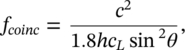

where h is the thickness, and c_L is the longitudinal wave speed in the panel (see Section 3.16). The critical frequency f_c may be considered to be the lowest possible value of the coincidence frequency and is related to sound waves at grazing incidence (θ = 90°). We notice that because c_l is related to stiffness, the greater the stiffness, the lower the coincidence frequency.

If the panel is excited by a plane sound wave so that the trace wavelength λ_T = λ/sinθ ≠ λ_b (see Figure 3.26), a forced wave, not a free wave, will be created on the panel. This forced wave will have a trace‐wavelength λ/sinθ and will travel at the trace‐wave speed c/sinθ. We have already calculated the sound transmitted by the panel in the mass‐law frequency region assuming forced waves in Section 12.2.1. Cremer first published a theory which accounted for the coincidence effect in sound transmission [11]. However, his theory assumes that the panel is infinite, and only single‐leaf partitions are discussed. Real partitions are, of course, finite, and this causes added complications in the theoretical models because we have to take into account bending‐wave reflections at the panel boundaries. Careful theoretical study of this case shows that for free vibration of a finite panel only certain discrete frequencies can exist. These frequencies are known as the resonance or natural frequencies, and their values depend on the spatial boundary conditions (edge constraints) of the panel. In Section 2.4.2 of this book we showed that each natural frequency is associated with a pattern of vibration on the panel, known as a mode shape. These modes of vibration are sometimes known as “standing” waves since they appear to stand still. In reality, each mode or standing wave on a panel is composed of the summation of four traveling waves.

Although Eq. (3.85) (and Eq. (12.23) for θ = 90°) is still valid on a finite panel, the finite size of a panel causes some changes from the previous discussions. Now, below the critical frequency a panel can radiate sound (although inefficiently). Also, coincidence can still occur (above) the critical frequency, when wave matching occurs between acoustic trace wavelengths and free‐bending wavelengths. Above the critical frequency, the sound transmission tends to be dominated by resonant motion on the panel and not by forced motion. In this region, panel damping is important and can alter the panel TL.

For frequencies greater than the critical frequency, the TL can be predicted by the empirical field incidence expression [9, 10]

(12.24)

where TL₀(f_c) is the transmission loss for normal incidence at the critical frequency and η is the damping loss factor of the panel (see Section 2.5.2 of this book). We see in Eq. (12.24) how the TL above the critical frequency is governed by the damping of the panel. If the frequency is kept constant, then each time the damping loss factor of the panel is doubled, the TL increases by 10 log (2) = 10(0.301) ≈ 3 dB. For a fixed damping and fixed mass per unit area M, the TL increases by 33.22 log (2) = 33.22(0.301) ≈ 10 dB for each doubling of frequency (octave) (see Figure 12.4).

Below the critical frequency, trace wave matching cannot occur for free waves on the panel, and the forced transmission dominates. Although this discussion is necessarily simplified, it explains the experimentally observed results for TL of panels.

EXAMPLE 12.4

Calculate the normal‐incidence mass law for a 18‐mm thick aluminum panel (c_l = 5420 m/s and density 2667 kg/m³) at a frequency of 500 Hz. Also determine the random‐incidence and field‐incidence mass laws. What is TL_field at 2800 Hz when η = 0.01?

SOLUTION

The mass per unit area of the panel is M = 2667 × 18 × 10⁻³ = 48 kg/m². The normal‐incidence mass law is calculated by Eq. (12.14)

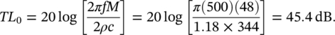
Using Eq. (12.22a) the random‐incidence is TL_rand = TL₀ − 10log(0.23 × TL₀) = 45.4 − 10log(10.442) = 35.2 dB. The field‐incidence mass law is given by Eq. (12.22c): TL_field = 20log(Mf) − 47 = 20log (48 × 500) − 47 = 40.6 dB.

The critical frequency of the panel is determined from Eq. (12.23) for θ = 90°,

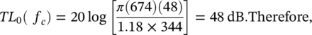
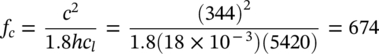 Hz. Since f = 2800 Hz is greater than the critical frequency, the field‐incidence TL is determined using Eq. (12.24). First,

So far we have only discussed the transmission of sound through single‐leaf partitions. The transmission of sound through double‐leaf partitions is discussed in the following section.