Classical Reactive Muffler Theory

10.6.1 Transmission Line Theory

We will first make some simplifying assumptions:

1. Sound pressures are small compared with the mean pressure
2. There are no mean temperature gradients or mean flow, and
3. Viscosity can be neglected.

If plane waves are assumed to exist in a muffler element (see Figure 10.9) then the sound pressure p anywhere in the muffler element can be represented as the sum of right and left traveling waves p⁺ and p⁻ respectively

(10.2a)

(10.2b)

(10.3a)

(10.3b)

(10.3c)

Note that p and V represent the magnitude (and phase) of the total sound pressure and volume velocity. The time dependence (constant multiplying factor e^jωt) has been omitted for brevity. The right and left traveling sound waves are represented by the + and − superscripts, respectively, while P represents the pressure amplitude; S the cross‐sectional area, ρc/S the characteristic acoustic impedance (traveling wave pressure divided by traveling wave volume velocity), k = ω/c, the acoustic wavenumber, ω the angular frequency, c the speed of sound, and ρ the fluid density.

10.6.2 TL of Resonators

Davis et al. used theory such as this to predict the TL of various resonator chamber type mufflers [21, 22] by assuming: (i) continuity of pressure and (ii) continuity of volume velocity at discontinuities.

a) TL of Expansion Chambers

For example, if there is a sudden increase in area at station l and a sudden decrease in area (see Figure 10.9) at station 2, then the resulting chamber formed is known as an expansion chamber (see Figure 10.10) and its TL can be found as follows.

The chamber TL is easily derived from Eqs. (10.2a) to (10.3c) above by assuming that the sudden area changes occur at x = 0 and x = l (resulting in the area change ratio, m) and by assuming the continuity of pressure and volume velocity at the area discontinuities [21, 22]. In the inlet pipe, P₁ ⁺ and P₁ ⁻ are the pressure amplitudes of the right and left traveling waves incident and reflected at the expansion chamber entrance.

Using Eqs. (10.2a) through (10.3c), the sound pressure and volume velocity in the inlet pipe 1 are:

(10.4a)

and

(10.4b)

The sound pressure and volume velocity in the expansion chamber 2 are:

(10.5a)

and

(10.5b)

The sound pressure and volume velocity in the outlet pipe 3 (assuming anechoic conditions with no reflections) are:

(10.6a)

and

(10.6b)

The boundary conditions of continuity of sound pressure p and volume velocity V at the pipe junctions x = 0 and x = l give:

At x = 0:

(10.7a)

and

(10.7b)

At x = l:

(10.8a)

and

(10.8b)

For a given expansion chamber length l and wavenumber k, there are four Eqs. (10.7a), (10.7b), (10.8a), and (10.8b) five unknown complex sound pressure amplitudes P₁⁺, P₁⁻, P₂⁺, P₂⁻, and P₃⁺. These equations can be solved simultaneously (putting S₂/S₁ = m), to give:

(10.9)

For plane waves, the ratio of the incident sound intensity at the expansion chamber entrance to the transmitted intensity at the outlet (in the tailpipe) assuming anechoic conditions in the tailpipe given by:

(10.10)

and thus, the TL is

(10.11)

which from Eq. (10.10) becomes

(10.12)

Figure 10.11 gives a plot of Eq. (10.12)

EXAMPLE 10.1

A compressor is pumping air with a gas temperature of 84 °C. The fundamental pumping frequency is 6000 rpm. Noise at the fundamental frequency is a problem. Design an expansion chamber with the shortest length suitable to suppress the exhaust noise. The inlet and outlet tube diameters are 5.0 cm (≈2.0 in.)

SOLUTION

The speed of sound c at 84 °C is (see Eq. (3.3)): c = 331.6 + 0.6 × 84 = 382 m/s.

Assume the pump noise is predominantly at the pumping frequency of 6000/60 = 100 Hz.

The wavelength λ = 382/100 = 3.82 m. For the shortest length chamber, kl = π/2 and so l = π/2 k = π/2 (2π/λ) = λ /4 = 3.82/4 = 0.955 m. Interpolating between the curves in Figure 10.11, select m = 12.

To calculate the TL for m = 12, Eq. (10.12) is used, with sin kl = sin π/2 = 1. Thus, TL for (m = 12) = 10 log[1 + ¼ (12 – 1/12)²] = 10 log[1 + ¼ (12 – 0.083)²] = 10 log[1 + ¼ (11.92)²] = 10 log[1 + 142/4] = 10 log[36.5] = 15.6 dB. For a circular cross‐section chamber with m = 12, the chamber diameter d = 5.0 × √12 = 5 × 3.46 = 17.3 cm.

In order to obtain exact values for the expansion ratio m, and chamber diameter d, a quadratic equation must be solved. Writing Eq. (10.12) with kl = π/2

and m − 1/m = n, which gives (1/m) [(m² − nm) − 1] = 0. Writing n = 2 (10^TL/10 – 1)^1/2, we have the solution for n in the quadratic

and for TL = 15 dB,

The negative root to the quadratic has no practical meaning, so the chamber diameter becomes:

An expansion chamber diameter of 17.3 cm instead of 16.7 cm will give a small increase in TL of 0.6 dB.

b) TL Caused by a Side‐Branch

Figure 10.12 shows a pipe with a side‐branch located at x = 0.

In the inlet pipe (to the left of the side‐branch), the pressure and volume velocity are

(10.13)

(10.14)

and

(10.15)

(10.16)

At the branch junction, where (x = 0), the sound pressure and volume velocity are assumed to be continuous, so that

(10.17)

where p_b is the pressure at the mouth branch and p_t is the transmitted pressure in pipe 3. Continuity of volume velocity gives:

(10.18)

where V_t is the transmitted volume velocity in pipe 3, assuming anechoic conditions in the tailpipe, pipe 3. Writing S₁ = S₃ = S,

(10.19)

and V_b = p_b/Z_b and dividing Eqs. (10.18) by (10.17), and using the relations in Eq. (10.19), we obtain:

(10.20)

which gives

(10.21)

where the Z, Z_t, and Z_b represent the system input, output, and branch impedances respectively (ratios of sound pressure to volume velocity). Figure 10.13 shows an electrical analogy of Eq. (10.21).

(10.22)

and

(10.23)

After rearrangement, we write the transmission coefficient α_t as

(10.24)

where Z_b = R_b + jX_b and R_b and X_b are the real and imaginary parts of the impedance Z_b. The TL is then:

(10.25)

c) Helmholtz Resonator

Consider a container of volume V_hr connected to a neck of length l. This is called a Helmholtz resonator (see Figure 10.14).

The acoustical behavior of Helmholtz resonators is well known. Their use in noise control applications where good low‐frequency sound absorption is required at a particular frequency is discussed in Chapter 8 of this book. The gas in the neck acts as a mass at low frequency and vibrates against the stiffness of the gas in the volume. Since the gas at each end of the neck of length l will also move, it is normal to add an end connection ∆l at each end making the effective neck length l’ = l + 2∆l.

The acoustic mass can thus be written as M = ρS_b l′. The acoustic stiffness K can be written as K = ρc² S_b ² /V_hr, where S_b is the neck cross‐sectional area, and V_hr is the resonator volume. The equation of motion of the gas in the neck is

(10.26)

and rearranging and assuming simple harmonic motion (but omitting the time variation e^jωt),

(10.27)

Thus, the impedance is

(10.28)

Setting R_b = 0, the impedance becomes:

(10.29)

The natural frequency of the Helmholtz resonator is obtained when the reactive impedance is zero, thus

(10.30)

where V_hr is the volume of the Helmholtz resonator.

EXAMPLE 10.2

A 400 ml bottle has a 2.5 cm (≈1 in.) diameter neck, which has an effective length l′ of 6 cm. What is its resonance frequency when it is excited by blowing?

SOLUTION

It is seen that the resonance frequency is just 9 Hz lower than lower C on the piano or violin (256 Hz). This frequency is one octave lower than middle C (512 Hz). We note that the resonance frequency can be increased by reducing the volume in the bottle by adding water. To reach a note close to middle C (512 Hz), the volume would need to be reduced to 100 ml by adding 300 ml of water.

d) Helmholtz Resonator as a Side‐Branch

Substituting R_b = 0 and the reactance X_b given by Eq. (10.29) into Eqs. (10.24) and (10.25) gives the TL:

(10.31)

We note that the TL → ∞ at the resonance frequency f_r = (c/2π)√(S_b/l′V_hr). This type of side‐branch resonator produces a useful broadband attenuation around this frequency. Davis et al. [22, 23, 64] give a series of curves for the side‐branch Helmholtz resonator after Eq. (10.31) is reorganized with f/f_r as a parameter.

EXAMPLE 10.3

Calculate the TL of the Helmholtz resonator as a side‐branch for a volume of V_hr = 0.00112 m³, l = 6 mm (≈1/4 in.), S_b = 7.5 × 10⁻⁴ m², S = 2.8 × 10⁻³ m² over the range from 0 to 500 Hz. Assume l′ = l + 0.85a, where a is the branch tube radius.

SOLUTION

If S_b = 7.5 × 10⁻⁴ m² = 7.5 cm², then a² = 7.5/π, a = 1.55 cm. Now, l′ = 0.006 + 2 × (0.85) × 0.0155 = 3.23 cm (assuming two end corrections). Substituting the given values for S, S_b, and V_hr into Eq. (10.31) and assuming c = 343 m/s and l′ = 3.23 cm, we obtain Figure 10.15. From Eq. (10.30) we obtain f_r = 249 Hz. We observe that the TL is greater than 10 dB over a 75 Hz frequency range.

e) Quarter‐Wave Resonator as a Side‐Branch

We obtain the input impedance Z_b of a quarter‐wave resonator tube by considering simple harmonic waves traveling in and out of the tube (length l, see Figure 10.16). Waves will be reflected at the rigid hard end at which the impedance p/S_bu_b will be infinity. The input impedance (provided losses are ignored and R_b = 0) is

(10.32)

The input impedance is zero when ωl/c = nπ/2, n = 1, 3, 5, … thus, when ω_n = nπc/2l, or f_n = nc/4l and l = nc/4f = nλ/4. Thus the input impedance of a quarter‐wave resonator as a side‐branch has multiple values of high TL (unlike the Helmholtz resonator). These are given by f_n = nc/4 l, n = 1, 3, 5, …

The TL of a quarter‐wave resonator as a side‐branch is obtained by substituting Z_b in Eq. (10.32) into Eq. (10.25) giving

(10.33)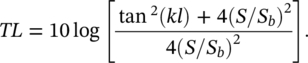

The TL is seen to depend upon frequency ω = kc or f = kc/2π and the ratio S/S_b.

EXAMPLE 10.4

Calculate the length l of the quarter‐wave resonator to make the first standing quarter‐wave frequency 700 Hz. Also calculate the frequency corresponding to three and five standing quarter‐waves.

SOLUTION

If f_n = nc/4 l, and putting n = 1, l = (1/f_n) × (1 × 343)/4 = 343/(700 × 4) = 0.1225 m. f_n for n = 3 is 3 × 700 = 2100 Hz and f_n for n = 5 is 5 × 700 = 3500 Hz.

EXAMPLE 10.5

Calculate the TL for the side‐branch quarter‐wave resonator for l = 0.2 m. Assume S_b = S = 5 × 10⁻⁵ m².

SOLUTION

If S_b = 2 × 10⁻³ m² = 20 cm², then a² = 20/π, a ≈ 2.5 cm. Assuming an effective length l + 0.85a, where a is the side‐branch tube radius, then l′ = 20 + 2.5(0.85) = 22.1 cm. Substituting the value for l = l′ and S/S_b = 1 into Eq. (10.33) gives the result in Figure 10.17. We note that when kl′ = nπ/2, n = 1, 3, 5, then the TL → ∞.

f) Orifice as a Side‐Branch

Consider a short length of pipe of length l as a branch. The pipe radius a and length l are assumed to be small compared to the wavelength λ. The real and imaginary parts of the branch impedance of the orifice pipe are

(10.34)

where the effective length of the short pipe is l′ = l + 2 × (0.85)a = = l + 1.7a.

The TL is

(10.35)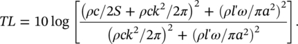

The ratio of acoustic resistance R_b to acoustic reactance X_b is

(10.36)

Since the tube length l and radius a are assumed to be much less than the wavelength λ, then ka → 0.

By neglecting losses in the orifice and setting R_b << X_b, the term ρck²/2π can be neglected. The TL becomes:

(10.37)

EXAMPLE 10.6

A small tube‐axial fan has eight blades and is running at a constant speed of 750 rpm. The fan is operating in a tube of inside diameter 100 mm and thickness 2 mm. A hole of diameter 30 mm is drilled in the tube’s wall far from the fan. If the speed of sound inside the tube is c = 344 m/s, determine the TL provided by this orifice as a side‐branch at the blade passing frequency (BPF) of the fan.

SOLUTION

The BPF of the fan is calculated using Eq. (11.7) as f = 8 × 750/60 = 100 Hz. Then, k = 2π(100)/344 = 1.8265 m⁻¹. Now, S = π(0.1/2)² = 0.0079 m² and a = 0.03/2 = 0.015 m. The effective length of the short pipe is l′ = 2 + 1.7 (15) = 27.5 mm = 0.0275 m. Since ka = 0.0274 << 1, we can use Eq. (10.37): TL = 10 log [1 + (π × 0.015²/2 × 0.0079 × 0.0275 × 1.8265))²] = 10 log [1 + 0.7933] = 10 log (1.7933) = 2.5 dB.

10.6.3 NACA 1192 Study on Reactive Muffler TL

The extensive study on reactive mufflers published by Davis et al. as NACA 1192 is a very important seminal work [21]. See also Ref. [64] in which Ref. [21] is reprinted. It was republished in Ref. [22] with additional material and discussion included. It has formed the basis of much subsequent research on reactive mufflers used on automobiles and in industry. Davis et al. studied 77 different mufflers. Measurements of TL (called attenuation by Davis et al.) were made on each one with a loudspeaker as a source and with a reflection‐free tailpipe termination. The results were compared with theory. The mufflers studied included expansion chambers, side‐branch resonators including Helmholtz resonators and combinations of these elements.

Figure 10.18a shows the effect of increasing the expansion ratio m from 4 to 16. It is seen that increasing m (see Eq. (10.12)) causes an increase in the peak TL. The plane wave theory fails above about 690 Hz, where cross modes begin to appear. Figure 10.18b shows the effect of keeping the ratio m constant, but increasing the muffler length. It is noted that the TL drops to zero when the muffler length ℓ is equal to one half a wavelength λ/2 or for frequencies f = nc/2ℓ. As the length ℓ increases, the first peak in the TL keeps constant at about 20 dB, but continually moves to a lower frequency. Further length increase results in additional peaks occurring.

Figure 10.19 shows the effect of connecting together two expansion chamber mufflers of the same expansion ratio m = 16. Figure 10.19a shows the effect of different length external connection tubes, while Figure 10.19b shows the effect of using different length internal connection tubes. Muffler 12, which appears in both Figure 10.19a and b, can be considered to have connection tubes of zero length. If a muffler 48 in. (1.25 m) long could be acceptable, muffler 19 could be used to provide about 30–40 dB attenuation over a broad frequency range up to 500 Hz.

Figure 10.20a shows the effect of using connecting tubes of length equal to the individual chamber lengths. The connecting tubes in each case are terminated at the center of each chamber.

Muffler 19 is shown in both Figures 10.19b and 10.20a. The mufflers in Figure 10.20a can all produce high broadband attenuation of 30 dB or more, but the shorter mufflers have a poorer performance than muffler 19 at frequencies below 200 Hz. Figure 10.20b shows the attenuation provided by side‐branch Helmholtz resonators of the same volume but with different diameter necks.

In Figure 10.21, Davis et al. investigated the performance of single‐chamber concentric resonators. In Figure 10.21a, the effect of varying the attenuation parameter  while keeping the chamber length constant is shown. Here c₀ is the conductivity, V the volume of the concentric resonator, and S the cross‐sectional area of the connecting tubes. Figure 10.21b shows the effect of varying the chamber length while keeping both the conductivity c₀ and the resonator volume constant.

Figure 10.22 shows the effect of varying the conductivity c₀ of the connecting elements (tubes or orifices) of double resonator mufflers while the volume V is kept constant. Figure 10.22a shows the effect of varying the conductivity c₀ when small tubes are used as the connecting elements between the exhaust tube and the concentric resonators. Figure 10.22b shows the effect when orifices are used as the connecting elements instead of small tubes. The considerable increase in the attenuation (TL) that occurs when orifices are used instead of small tubes is observed when the results of Figure 10.22b are compared with those in Figure 10.22a.

Figure 10.23 shows the attenuation (TL) of combination mufflers comprised of expansion chambers and concentric tube Helmholtz resonators. Mufflers 73 and 73R (shown in Figure 10.23) show that the order of the double chamber resonators is relatively unimportant. The two peaks are caused by the two different types of chamber. The attenuation caused by these mufflers is over a broad frequency range.

10.6.4 Transfer Matrix Theory

An alternative approach is to assume that the sound pressure p and volume velocity V at stations l and 2 in Figure 10.9 can be related by:

(10.38)

and

(10.39)

An electrical circuit analogy can be used where the pressure p is analogous to voltage and volume velocity V to current. This is known as the impedance analogy. Note that an alternative mobility analogy is sometimes used [5]. The circuit element can be represented by the four‐pole element shown in Figure 10.24. If the muffler section is simply a rigid straight pipe (See Figure 10.9.) of constant cross‐section, then from Eqs. (10.2b) and (10.3b), the sound pressure and volume velocity at stations l and 2 (x = 0 and x = L) are:

(10.40)

(10.41)

(10.42)

(10.43)

The parameters A, B, C, and D may be evaluated using a “black box” system identification technique. To evaluate A and C, assume that the matrix output terminals are open circuit, or V₂ = 0.

Then Eq. (10.43) gives P⁺/P⁻ = e^j2kL and Eqs. (10.38) and (10.39) give

Using this result for P⁺/P⁻, and Eqs. (10.40)–(10.42) after some manipulation, it is found that

Similarly, to evaluate B and D assume that the matrix output terminals are short‐circuited and p₂ = 0. Then Eq. (10.43) gives P⁺/P⁻ = e^j2kL and Eqs. (10.38) and (10.39) give

Using this result for P⁺/P⁻ and Eqs. (10.40), (10.42) and (10.43), it is found that

Substituting these results for A, B, C, and D into Eqs. (10.38) and (10.39) and writing them in matrix form gives

(10.44)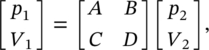

where the four‐pole constants (for a straight pipe of length L) are:

(10.45)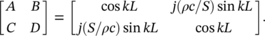

Note that AD – BC = 1. This is a useful check on the values derived of the four‐pole parameters and is a consequence of the fact that the system obeys the reciprocity principle [5]. The matrix in Eq. (10.45) relates the total sound pressure and volume velocity at two stations in a straight pipe.

If several component systems are connected together in series, as in Figure 10.25 then the transmission matrix of the complete system is given by the product of the individual system matrices:

(10.46)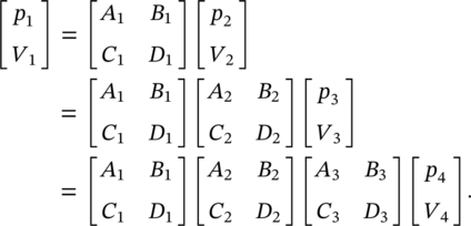

This matrix formulation is very convenient particularly where a digital computer is used. The four‐pole constants A, B, C, and D can be found easily for simple muffler elements such as expansion chambers and straight pipes as has just been shown (see Eq. (10.45)). They can also be found in a similar manner for more complex muffler shapes (reversing end chambers and reversing end‐chamber/Helmholtz resonator combinations) by the finite element method using the same black box identification technique mentioned above (by alternately setting p₂ = 0 and V₂ = 0).