Free Vibration – Undamped

By free vibration, we mean that the system is set into motion by some forces which then cease (at t = 0) and the system is then allowed to vibrate freely for t > 0 with no external forces applied. First we will consider a free undamped multi‐degree of freedom system, i.e. [R] = [0] and f(t) = 0. Therefore, Eq. (2.22) now becomes

(2.23)

Similarly to the case of the single‐degree‐of‐freedom system discussed in Section 2.3, we assume harmonic solutions in the form

(2.24)

where A is the vector of amplitudes. Substituting Eq. (2.24) into (2.23) yields

(2.25)

Equation (2.25) has a nontrivial solution if and only if the coefficient matrix ([K] − ω²[M]) is singular, that is the determinant of this coefficient matrix is zero,

(2.26).

Equation (2.26) is called the characteristic equation (or characteristic polynomial) which leads to a polynomial of order n in ω². The roots of this polynomial, denoted as  (for i = 1, 2, …, n), are called the characteristic values (or eigenvalues). The square root of these numbers, ω_i are called the natural frequencies of the undamped multi‐degree of freedom system and they can be arranged in increasing order of magnitude by ω₁ ≤ ω₂ ≤ … ≤ ω_n. The lowest frequency ω₁ is referred to as the fundamental frequency. The characteristic equation has only real roots due to the symmetry of the mass and stiffness matrices. In general, all the roots are distinct except in degenerate cases.

Note that  are the eigenvalues of the matrix [M]⁻¹[K], where [M]⁻¹ is the inverse of [M]. Associated with each characteristic value , there is an n‐dimensional column linearly independent vector called the characteristic vector (or eigenvector) A_i which is referred to as the i‐th natural mode (normal mode, principal mode or mode shape) [10–13]. A_i is obtained from the homogeneous system of equations represented by Eq. (2.27) as

(2.27).

Since the system of equations represented by Eq. (2.27) is homogeneous, the mode shape is not unique. However, if  is not a repeated root of the characteristic equation then there is only one linearly independent nontrivial solution of Eq. (2.27). The eigenvector is unique only to an arbitrary multiplicative constant [13]. It can be shown that the mode shapes are orthogonal. This property is important and allows a set of n decoupled differential equations of motion of a multi‐degree of freedom system to be obtained by using a modal transformation [10].

Solving Eq. (2.27) and replacing it into Eq. (2.24), we obtain a set of n linearly independent solutions q_i = A_i exp{jω_i t} of Eq. (2.23). Thus, the total solution can be expressed as a linear combination of them,

(2.28)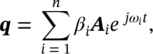

where β_i are arbitrary constants which can be determined from initial conditions [usually with initial displacements and velocities q(t = 0) and ]. Equation (2.28) represents the superposition of all modes of vibration of the multi‐degree of freedom system.

EXAMPLE 2.5

It is illustrative to consider an example of a two‐degree‐of‐freedom system, as the one shown in Figure 2.11, because its analysis can easily be extrapolated to systems with many degrees of freedom.

SOLUTION

The two‐coordinates x₁ and x₂ uniquely define the position of the system illustrated in Figure 2.11 if it is constrained to move in the x‐direction. The equations of motion of the system are:

(2.29a)

and

(2.29b)

We observe that the equations of motion are coupled, that is to say the motion x₁ is influenced by the motion x₂ and vice versa. Equation (2.29) can be written in matrix form as

(2.30)

where q = ,  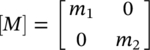and .

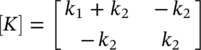Equation (2.26) gives the characteristic equation

(2.31)

For simplicity, consider the situation where m₁ = m₂ = m and k₁ = k₂ = k. Then, Eq. (2.31) becomes

(2.32)

Solving Eq. (2.32) gives the natural frequencies of the system as

(2.33)

Note that Eq. (2.32) has four roots, the additional two being −ω₁ and −ω₂. However, since these negative frequencies have no physical meaning, they can be ignored. For each positive natural frequency there is an associated eigenvector that is obtained from Eq. (2.27). Substitution of Eq. (2.33) into Eq. (2.27) and solving for A_i, yields:

(2.34a)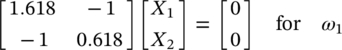

and

(2.34b)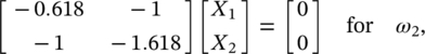

where X₁ and X₂ are the elements of vector A_i. Equations (2.34a) and (2.34b) are homogenous, so that no unique solution is possible. Indeed, a solution with all its components multiplied by the same constant is also a solution [11]. Choosing arbitrarily X₁ = 1 and solving Eq. (2.34) we get the eigenvectors

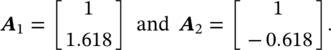
When used to describe the motion of a multi‐degree of freedom system, the mode shape refers to the amplitude ratio. These ratios are possible to obtain because their absolute values are arbitrary [12]. Thus, we express the mode shapes as the ratio of the amplitudes X₁/X₂. Then, for ω₁, X₁/X₂ = 0.618 and for ω₂, X₁/X₂ = −1.618. These ratios can be represented in the mode plot of Figure 2.12. We note that when this simple two‐degree of freedom system vibrates at the first (fundamental) natural frequency ω₁, the two masses vibrate in phase (Figure 2.12a). When the system vibrates at the second natural frequency ω₂, the two masses vibrate out of phase (Figure 2.12b).