Frequency Analysis Using Filters

Sound and vibration signals can be combined, but they can also be broken down into frequency components as shown by Fourier over 200 years ago. The ear seems to work as a frequency analyzer. We also can make instruments to analyze sound signals into frequency components.

In order to determine experimentally the contribution of the overall signal in some particular frequency band we filter the signal. Most of the important points concerning filters can be observed from a simple R–C passive circuit. By passive we mean that no electrical power is supplied. However, practical filters are usually made from more complicated R–C passive filters or active filters, involving R–C components, inductances, amplifiers, and a power supply. Modern digital signal processing can also be used to filter a signal. Digital filters are implemented through a series of digital operations (addition, multiplication, and time delay) on a digitized signal [3, 5, 14].

In a high‐pass filter, only high‐frequency signals are passed without attenuation. An ideal high‐pass filter would pass no signal below the cutoff frequency and would have a vertical “skirt,” which is impossible to achieve by use of a simple RC passive filter. Practical high‐pass filters have more complicated circuits and normally incorporate inductances and/or active components. High‐pass filters are often used when the displacement signal from a transducer is analyzed. This is because frequently the high‐frequency displacement is of interest and large amplitude low‐frequency signals must be filtered out to prevent the dynamic range of the instrumentation from being exceeded.

In a low‐pass filter only low‐frequency signals are passed without attenuation. In practice, the skirt of a simple RC filter is usually not steep enough and a more complicated circuit is also needed. In modern noise and vibration instrumentation, low‐pass filters are often used as anti‐aliasing filters at the input of an analog‐to‐digital converter (ADC) to suppress unwanted high‐frequency signals. Aliasing errors occur when signals at high frequency (above the upper frequency limit) are interpreted as lower frequency signals below the upper frequency limit.

In a band‐stop (or band‐rejection) filter most frequencies are passed without attenuation; but those frequencies in a specific range are attenuated to very low levels. It is the opposite of a band‐pass filter. Band‐stop filters are commonly used as anti‐hum filters and to remove specific interference frequencies in a complex signal.

By combining the simple high‐pass and low‐pass filters, a simple band‐pass filter is produced. In a band‐pass filter all simple harmonic frequency signals within a band are passed with little, if any, attenuation. All signals outside this band are attenuated. In practice it is usually desirable to make the skirts of such a filter steeper. This requires the use of additional electrical circuit elements and/or the use of active filters. Figure 1.9 illustrates the filtering process and shows only the magnitude of the signals in the frequency domain [10].

Band‐pass filters are frequently used in acoustics and vibration. A frequency weighting network such as A‐weighting is a special kind of band‐pass filter. Frequency analysis using band‐pass filters is commonly carried out using (i) constant frequency band filters and (ii) constant percentage filters. The following symbol notation is used in the characterization of a band‐pass filter: f_L and f_U are the lower and upper cutoff frequencies, and f_C and Δf are the band center frequency and the frequency bandwidth, respectively. Thus Δf = f_U − f_L. See Figure 1.10.

In constant bandwidth filters, the bandwidth Δf = f_U − f_L is kept constant regardless of the setting of the filter center frequency.

The constant percentage filter (usually one‐octave or one‐third‐octave band types) most parallels the way the human auditory system analyzes sound and, although digital processing has mostly overtaken analog processing of signals, it is still frequently used. The human audible range is spanned by just a few octaves, so octave analysis produces a relatively coarse classification. Resolution can be improved by breaking each octave band into fractional‐octave bands, which preserves the logarithmic band spacing. Thus, if the frequency scale is divided into contiguous frequency bands, the ratio f_U/f_L is the same for each band. The center frequency f_C for each band is defined as the geometric mean which is in the middle between f_L and f_U on a logarithmic frequency scale and is always less than the arithmetic average. Thus, the ratio of center frequencies of contiguous bands is the same as f_U/f_L for any one band. Octave and third‐octave band filters are widely used, in particular for acoustical measurements [12].

a) One‐Octave Bands

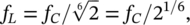
For one‐octave bands, the cutoff frequencies f_L and f_U are defined as follows:

The center frequency (or geometric mean) is . Thus f_U/f_L = 2.

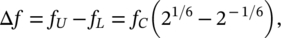
The bandwidth Δf is given by

so Δf ≈ 70% (f_C).

b) One‐Third‐Octave Bands

For one‐third‐octave bands, the cutoff frequencies, f_L and f_U, are defined as follows:

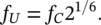
The center frequency (geometric mean) is given by . Thus f_U/f_L = 2^1/3.

The bandwidth Δf is given by

so Δf ≈ 23% (f_C).

We thus see clearly why the filter bands we have just discussed are called constant percentage. This is because the bandwidth is a constant percentage of the filter center frequency f_C. Of course, the filter bandwidth does not have to be defined in terms of a fraction of an octave but can be defined simply in terms of the percentage of the center frequency. Since it is impracticable to make measurements at a large number of fixed frequencies, noise measurements are made at a selected number of standardized frequencies called preferred center frequencies. Standard one-octave and one-third-octave band specifications take advantage of the fact that 2^10/3 ≈ 10. The ISO recommendation values for preferred center frequencies are given in Table 1.1 [15]. Specifications for octave‐band and fractional‐octave‐band filters are defined by the IEC 1260:1995 and the ANSI S1.11:2004 standards [16, 17].

Table 1.1 Preferred center frequencies for noise measurements according to ISO R 266 [15].

Preferredfrequencies, Hz	1/1oct.	1/3oct.	Preferredfrequencies, Hz	1/1oct.	1/3oct.	Preferredfrequencies, Hz	1/1oct.	1/3oct.
16	×	×	200		×	2500		×
20		×	250	×	×	3150		×
25		×	315		×	4000	×	×
31.5	×	×	400		×	5000		×
40		×	500	×	×	6300		×
50		×	630		×	8000	×	×
63	×	×	800		×	10 000		×
80		×	1000	×	×	12 500		×
100		×	1250		×	16 000	×	×
125	×	×	1600		×
160		×	2000	×	×

Note that:

1. The center frequencies of one‐octave bands are related by 2, and 10 frequency bands are used to cover the human hearing range. They have center frequencies of 31.5, 63, 125, 250, 500, 1000, 2000, 4000, 8000, 16 000 Hz.
2. The center frequencies of one‐third octave bands are related by 2^1/3 and 10 cover a decade of frequency, and thus 30 frequency bands are used to cover the human hearing range: 20, 25, 31.5, 40, 50, 63, 80, 100, 125, 160, …, 16 000 Hz.

Thus we note that at high frequencies a constant bandwidth analyzer will obviously have a narrower bandwidth than the constant percentage filter. Figure 1.11 shows a comparison of the bandwidths of constant percentage and constant band filters at the same frequencies.

EXAMPLE 1.5

Determine the percentage bandwidth of the center frequency of a 1/12‐octave band filter.

SOLUTION

1/12-octave filters are obtained by dividing each one-octave band into 12 geometrically equal sub‐sections, i.e. f_U/f_L = 2^1/12. By the same procedure as for octave and one‐third‐octave filters, we get the result that for 1/12‐octave bands the cutoff frequencies, f_L and f_U, are f_C × 2^−1/24 and f_C × 2^1/24, respectively. Then, the bandwidth is given by Δf = f_U − f_L = f_C(2^1/24 − 2^−1/24), so Δf ≈ 6% (f_C).

There are two main types of constant percentage filters in common use: (i) those with a fixed center frequency and bandwidth which is a certain percentage of the center frequency, and (ii) those with a variable (or tunable) center frequency and a bandwidth which can be set to certain selected percentages of the center frequency. The first type of filter is perhaps in most common use. In practical instruments, many different parallel filters each with a different center frequency are assembled in one unit. The instrument is provided with a root mean square detector and a display.

On the other hand, instruments for constant bandwidth filter analysis are normally constructed so that the center frequency of a single filter can be tracked effectively throughout the frequency range of interest. Often different bandwidth settings are available on the same instrument (e.g. 1, 5, 10, 20 Hz). The narrower the bandwidth chosen, the slower the tracking rate should be to obtain reliable results. A rule which should be used in spectrum analysis is that the duration, T, of the noise sample length (or of the analysis time) must be at least as long as the reciprocal of the bandwidth Δf,

(1.16)

This fundamental principle, also known as the uncertainty principle, puts a limit on the corresponding resolutions in the time and frequency domain, meaning that narrow resolution in one domain means wide resolution in the other domain [10].

If fine frequency resolution is not needed or if the signal is broadband in nature, then octave band readings are sufficient. One‐third octave band readings (or narrower) should be used if the signal spectrum is not smooth or if pure tones are present. For diagnostic work on machinery, it may be necessary to use constant bandwidth filters (e.g. if the fan blade passing frequency and its higher harmonics must be separated).

When changes in level and frequency of a signal occur in a short period of time, real‐time frequency analysis is required to observe rapid variations in the signal and showing the results on a continuously updated display. Real‐time analysis can be performed using a frequency analyzer made up of a set of parallel filters and a detector (see Figure 1.12). The input signal is previously conditioned in terms of level (gain/attenuation) and high‐ and/or low‐pass filtering. A digital analyzer will require an anti‐aliasing filter at the input before the ADC. The conditioner is then connected to a large number of parallel band‐pass filter channels (usually between 30 and 40 for a standard one‐third octave band model). The detector detects the power in the transmitted signal in terms of its mean square or rms value. In Figure 1.12, only one detector is shown, and this is supposed to work as detector for all the filters in the situation of a parallel filter bank [10].