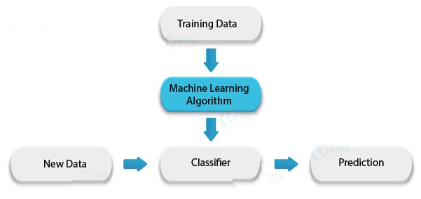
Naive Bayes Theorem

Naive Bayes is a powerful supervised learning algorithm that is used for classification. The Naive Bayes classifier is an extension of the above discussed standard Bayes Theorem. In a Naive Bayes, we calculate the probability contributed by every factor.

Most we use it in textual classification operations like spam filtering. Let us understand how Naive Bayes calculates the probability contributed by all the factors.

Suppose that, as a data scientist, you are tasked with developing a spam filter. You are provided with a list of spam keywords such as

• Free
• Discount
• Full Refund
• Urgent
• Weight Loss

However, the company you are working with is a product finance company. Therefore, some of the vocabulary occurring in the spam mails is used in the mails of your company. Some of these words are –

• Important
• Free
• Urgent
• Stocks
• Customers

You also have the probability of word usages in spam messages and company emails.

Spam Email	Company Email
Free (0.3)	Important (0.5)
Discount (0.15)	Free (0.25)
Full Refund (0.1)	Urgent (0.1)
Urgent (0.2)	Stocks (0.5)
Weight Loss (0.25)	Customers (0.1)

Suppose you obtain have a message “Free trials for weight loss program. Become members at a discount.” Is this message spam or a company email? Calculating the probability of the components occurring in the sentence – Free (0.4) + Weight Loss (0.25) + Discount (0.15) = 0.8 or 80%

Whereas, calculating the probability of it being an email from your company = Free (0.25) = 0.25 or 25%.

Therefore, the probability of the mail being spam is much higher than a company email.

A Naive Bayes Classifier selects the outcome of the highest probability, which in the above case was the feature of spam.

The Naive Bayes is referred to as ‘naive’ because it assumes the features to be independent of each other. The features in our example were the input words that are present in the sentence.

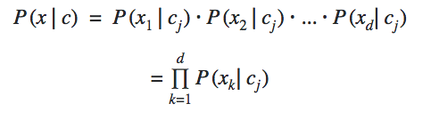
The conditional independence among all the features gives us the formula above. The frequency of the occurrence of features from x1 to xdis calculated based on their relation to the class cj.

Along with the prior probability and the probability of the occurrence of an event, we calculate the posterior probability through which we are able to find the probability of the object belonging to a particular class.

Along with this Bayes’ Theorem, Data Scientists use various different tools. You must check the different tools used by a Data Scientist.

Using Naive Bayes as a Classifier

In this section, we will implement the Naive Bayes Classifier over a dataset. The dataset used in this example is the Pima Indian Dataset which is an open dataset available at the UCI Library.

• In the first step, we import all the libraries that will allow us to implement our Naive Bayes Classifier and help us in wrangling the data.

import pandas as pd
from sklearn.model_selection import train_test_split
from sklearn.metrics import accuracy_score
from sklearn.naive_bayes import GaussianNB

• We then read the csv file through an online URL using read_csv function provided by the Pandas library.

data = pd.read_csv("/home/admin1/DataFlair/Data/diabetes.csv")

• Then, we proceed to divide our data into dependent variable (Y) and independent variables(X) as follows –

X = data.iloc[:, 0:8].values

y = data.iloc[:, 8].values

• Using the head() function provided by the Pandas library, we look at the first five rows of our dataset.

data.head()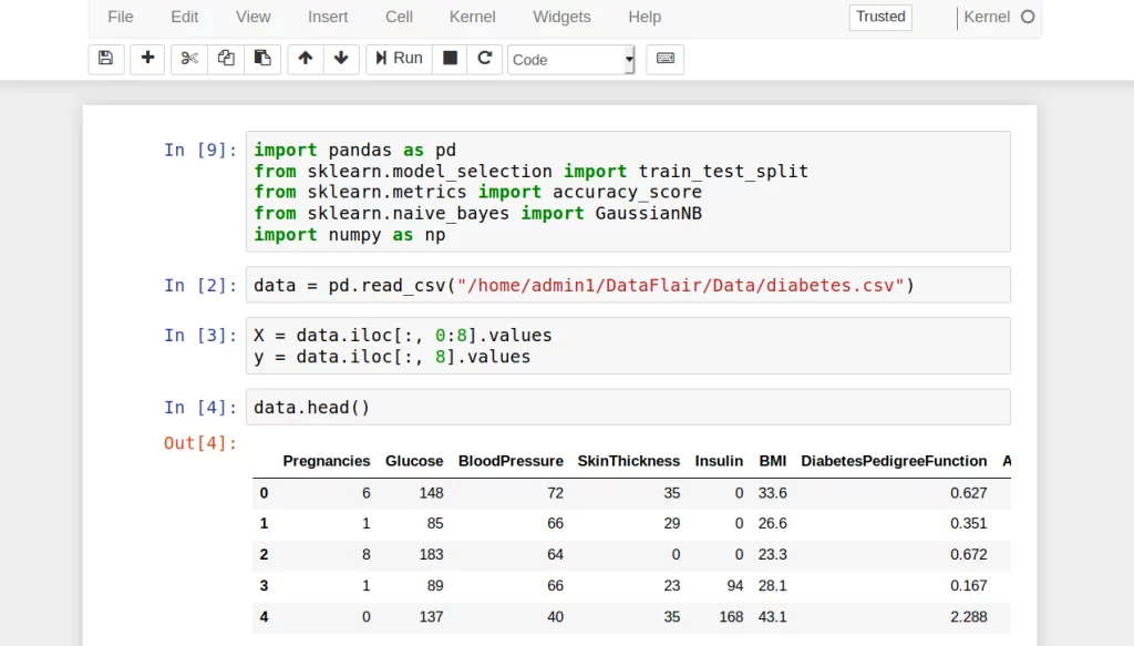

• We then proceed to split our dataset into training and validation sets. We will train our Naive Bayes Classifier on the training set and generate predictions from the test set. In order to do so, we will use the train_test_split() function provided by the sklearn library.

X_train, X_test, y_train, y_test = train_test_split(X, y, test_size=0.33, random_state=42)

• In this step, we apply the Naive Bayes Classifier and more specifically, the Gaussian Naive Bayes Classifier. It is an extension of the existing Naive Bayes Classifier that assumes the likelihood of the features to be Gaussian or normally distributed.

clf = GaussianNB()

clf.fit(X_train, y_train)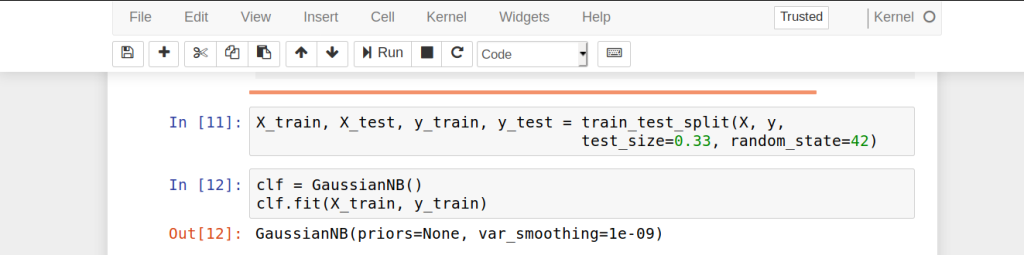

• In the next step, we generate predictions from our given test sample.

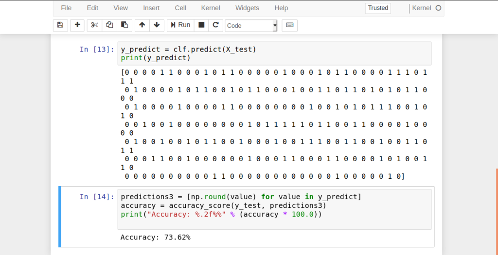
y_predict = clf.predict(X_test)

print(y_predict)

• Then, we measure the accuracy of our classifier. That is, we test to see how many values were predicted correctly.

predictions3 = [np.round(value) for value in y_predict]

accuracy = accuracy_score(y_test, predictions3)

print("Accuracy: %.2f%%" % (accuracy * 100.0))

Therefore, our Naive Bayes Classifier predicted 72.44% of the test-cases successfully.