3 Vibrating Systems

3.1 Mass–Spring System

a) Free Vibration – Undamped

Suppose a mass of M kilogram is placed on a spring of stiffness K newton‐metre (see Figure 2.5a), and the mass is allowed to sink down a distance d metres to its equilibrium position under its own weight Mg newtons, where g is the acceleration of gravity 9.81 m/s². Taking forces and deflections to be positive upward gives

(2.8)

Thus the static deflection d of the mass is

(2.8a)

The distance d is normally called the static deflection of the mass; we define a new displacement coordinate system, where Y = 0 is the location of the mass after the gravity force is allowed to compress the spring.

Suppose now we displace the mass a distance y from its equilibrium position and release it; then it will oscillate about this position. We will measure the deflection from the equilibrium position of the mass (see Figure 2.5b). Newton’s law states that force is equal to mass × acceleration. Forces and deflections are again assumed positive upward, and thus

(2.9)

Let us assume a solution to Eq. (2.9) of the form y = A sin(ωt + φ). Then upon substitution into Eq. (2.9) we obtain

We see our solution satisfies Eq. (2.9) only if

The system vibrates with free vibration at an angular frequency ω rad/s. This frequency, ω, which is generally known as the natural angular frequency, depends only on the stiffness K and mass M. We normally signify this so‐called natural frequency with the subscript n. And so

and from Eq. (3.2)

(2.10)

The frequency, f_n hertz, is known as the natural frequency of the mass on the spring. This result, Eq. (2.10), looks physically correct since if K increases (with M constant), f_n increases. If M increases with K constant, f_n decreases. These are the results we also find in practice.

EXAMPLE 2.2

A machine of mass 600 kg is mounted on four springs of stiffness 2 × 10⁵ N/m each. Determine the natural frequency of the system

SOLUTION

We model the system as a hanging spring‐mass system (see Figure 2.5). Equation (2.9) governs the displacement of the machine from its static‐equilibrium position. Since we have four equal springs, the equivalent stiffness is 4 × 2 × 10⁵ = 8 × 10⁵ N/m. The natural frequency is then determined using Eq. (2.10) as

We have seen that a solution to Eq. (2.9) is y = A sin(ωt + ϕ) or the same as Eq. (2.3). Hence we know that any system that has a restoring force that is proportional to the displacement will have a displacement that is simple harmonic. This is an alternative definition to that given in Section 2.2 for simple harmonic motion.

b) Free Vibration – Damped

Many mechanical systems can be adequately described by the simple mass–spring system just discussed above. However, for some purposes it is necessary to include the effects of losses (sometimes called damping). This is normally done by including a viscous damper in the system (see Figure 2.6). See Refs. [8, 9] for further discussion on passive damping. With viscous or “coulomb” damping the friction or damping force F_d is assumed to be proportional to the velocity, dy/dt. If the constant of proportionality is R, then the damping force F_d on the mass is

(2.11)

and Eq. (2.9) becomes

(2.12)

or equivalently

(2.13)

where the dots represent single and double differentiation with respect to time.

The solution of Eq. (2.13) is most conveniently found by assuming a solution of the form: y is the real part of A e^jλt where A is a complex number and λ is an arbitrary constant to be determined. By substituting y = A e^jλt into Eq. (2.13) and assuming that the damping constant R is small, R < (4MK)^1/2 (which is true in most engineering applications), the solution is found that:

(2.14)

Here ω_d is known as the damped “natural” angular frequency:

(2.15)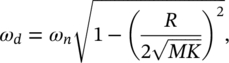

where ω_n is the undamped natural frequency . The motion described by Eq. (2.14) is plotted in Figure 2.7.

The amplitude of the motion decreases with time unlike that for undamped motion (see Figure 2.3). If the damping is increased until R equals (4MK)^1/2, the damping is then called critical, R_crit = (4MK)^1/2. In this case, if the mass in Figure 2.6 is displaced, it gradually returns to its equilibrium position and the displacement never becomes negative. In other words, there is no oscillation or vibration. If R > (4MK)^1/2, the system is said to be overdamped.

The ratio of the damping constant R to the critical damping constant R_crit is called the damping ratio δ:

(2.16)

In most engineering cases, the damping ratio, δ, in a structure is hard to predict and is of the order of 0.01–0.1. There are, however, several ways to measure damping experimentally [8, 9].

EXAMPLE 2.3

A 600‐kg machine is mounted on springs such that its static deflection is 2 mm. Determine the damping constant of a viscous damper to be added to the system in parallel with the springs, such that the system is critically damped.

SOLUTION

The static deflection is given by Eq. (2.8a) as d = Mg/K. Therefore K = Mg/d = 600(9.8)/2 × 10⁻³ = 294 × 10⁴ N/m. The system is critically damped when the damped constant R_crit = (4MK)^1/2 = (4 × 600 × 294 × 10⁴)^1/2 = 84 000 Ns/m.

(c) Forced Vibration – Damped

If a damped spring–mass system is excited by a simple harmonic force at some arbitrary angular forcing frequency ω (see Figure 2.8), we now obtain the equation of motion Eq. (2.17):

(2.17)

The force F is normally written in the complex form for mathematical convenience. The real force acting is, of course, the real part of F or |F| cos(ωt), where |F| is the force amplitude.

If we assume a solution of the form y = A e^jωt then we obtain from Eq. (2.17):

(2.18)

We can write A = |A| e^jα, where α is the phase angle between force and displacement. The phase, α, is not normally of much interest, but the amplitude of motion |A| of the mass is. The amplitude of the displacement is

(2.19)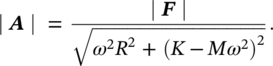

This can be expressed in alternative form:

(2.20)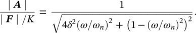

Equation (2.20) is plotted in Figure 2.9. It is observed that if the forcing frequency ω is equal to the natural frequency of the structure, ω_n, or equivalently f = f_n, a condition called resonance, then the amplitude of the motion is proportional to 1/(2δ). The ratio |A|/(| F|/K) is sometimes called the dynamic magnification factor (DMF). The number |F|/K is the static deflection the mass would assume if exposed to a constant nonfluctuating force |F|. If the damping ratio, δ, is small, the displacement amplitude A of a structure excited at its natural or resonance frequency is very high. For example, if a simple system has a damping ratio, δ, of 0.01, then its dynamic displacement amplitude is 50 times (when exposed to an oscillating force of |F| N) its static deflection (when exposed to a static force of amplitude |F| N), that is, DMF = 50.

Situations such as this should be avoided in practice, wherever possible. For instance, if an oscillating force is present in some machine or structure, the frequency of the force should be moved away from the natural frequencies of the machine or structure, if possible, so that resonance is avoided. If the forcing frequency f is close to or coincides with a natural frequency f_n, large amplitude vibrations can occur with consequent vibration and noise problems and the potential of serious damage and machine malfunction.

The force on the idealized damped simple system will create a force on the base . Substituting this into Eq. (2.17) and rearranging and finally comparing the amplitudes of the imposed force |F| with the force transmitted to the base |F_B| gives

(2.21)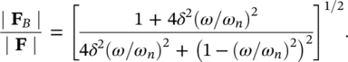

Equation (2.21) is plotted in Figure 2.10. The ratio |F_B|/| F| is sometimes called the force transmissibility T_F. The force amplitude transmitted to the machine support base, F_B, is seen to be much greater than 1, if the exciting frequency is at the system resonance frequency. The results in Eq. (2.21) and Figure 2.10 have important applications to machinery noise problems that will be discussed again in detail in Chapter 9 of this book.

Briefly, we can observe that these results can be utilized in designing vibration isolators for a machine. The natural frequency ω_n of a machine of mass M resting on its isolators of stiffness K and damping constant R must be made much less than the forcing frequency ω. Otherwise, large force amplitudes will be transmitted to the machine base. Transmitted forces will excite vibrations in machine supports and floors and walls of buildings, and the like, giving rise to additional noise radiation from these other areas.

Chapter 9 of this app gives a more complete discussion on vibration isolation.

EXAMPLE 2.4

What is the maximum stiffness of an undamped isolator to provide 80% isolation for a 300‐kg machine operating at 1000 rpm?

SOLUTION

The excitation frequency is f = 1000/60 = 16.7 Hz, or ω = 1000 × (2π/60) = 104.7 rad/s. For 80% isolation the maximum force transmissibility is 0.2.

Using Eq. (2.21) with δ = 0 and noting that isolation only occurs when  we get that 0.2 ≥ [(ω/ω_n)² − 1]⁻¹ which is solved giving ω/ω_n ≥ 2.45. This result can be also obtained from Figure 2.10. Therefore, the system’s maximum allowable natural frequency is f_n = 6.8 Hz, or ω_n = ω/2.45 = 104.7/2.45 = 42.7 rad/s. Consequently, the maximum isolator stiffness is K = Mω_n² = (300) × (42.7)² = 5.47 × 10⁵ N/m.